
Computer System Organization and Programming
CS 3410 - Fall 2025 taught by Giulia Guidi and Kevin Laeufer
| Lecture: MoWe 1:25pm-2:40pm ET, Uris Hall G01 | |
| Prelim: October 9, 2025 7:30 PM ET | Makeup Prelim: October 16, 2025 5:30 PM ET |
| Final: December 13, 2025 7:00 PM ET | Makeup Final: December 12, 2025 9:00 AM ET |
| Week | Date | Lecture | Lab | Assignment |
|---|---|---|---|---|
| 1 | Mon 8/25 | Lab 1: Nice to C You |
|
|
| Wed 8/27 | ||||
| 2 | Mon 9/1 |
|
Lab 2: Minifloat |
|
| Wed 9/3 | ||||
| 3 | Mon 9/8 | Lab 3: Huffman |
|
|
| Wed 9/10 | ||||
| 4 | Mon 9/15 | Lab 4: C & GDB Review |
|
|
| Wed 9/17 | ||||
| 5 | Mon 9/22 | Lab 5: CPU Simulator |
|
|
| Wed 9/24 |
|
|||
| 6 | Mon 9/29 | Lab 6: Assembly |
|
|
| Wed 10/1 | ||||
| 7 | Mon 10/6 | Lab 7: Assembly Functions |
|
|
| Wed 10/8 | ||||
| 8 | Mon 10/13 |
|
Lab 8: Buffer Overflow |
|
| Wed 10/15 |
|
|||
| 9 | Mon 10/20 | Lab 9: Cache Simulator |
|
|
| Wed 10/22 | ||||
| 10 | Mon 10/27 | Optional Lab (A9 worksheet review) |
|
|
| Wed 10/29 | ||||
| 11 | Mon 11/3 | Lab 10: Shall |
|
|
| Wed 11/5 | ||||
| 12 | Mon 11/10 | Optional Review Lab (Review: Calling Convention, Caches, Virtual Memory) |
|
|
| Wed 11/12 | ||||
| 13 | Mon 11/17 | Lab 11: Concurrent Hash Table |
|
|
| Wed 11/19 | ||||
| 14 | Mon 11/24 | No Lab (Thanksgiving) |
|
|
| Wed 11/26 |
|
|||
| 15 | Mon 12/1 | Lab 12: Raycasting (mandatory, even though A12 is optional) |
|
|
| Wed 12/3 | ||||
| 16 | Mon 12/8 | Final Review |
|
Syllabus
CS 3410, “Computer System Organization and Programming,” is your chance to learn how computers really work. You already have plenty of experience programming them at a high level, but how does your code in Java or Python translate into the actual operation of a chunk of silicon? We’ll cover systems programming in C, assembly programming in RISC-V, the architecture of microprocessors, the way programs interact with operating systems, and how to correctly and efficiently harness the power of parallelism.
TL;DR
- Course communication will happen on Ed.
- Log in with your
netid@cornell.eduemail address. You should already have access. - You’re responsible for knowing everything that we post as announcements there. Ignore announcements at your own risk.
- Log in with your
- Homework hand-in and grading happens on Gradescope.
- There are 11 assignments.
- The deadline is usually Wednesday night at 11:59pm. See the schedule for details.
- You have 12 total “slip days” you can use throughout the semester. You may use up to 3 for a given assignment.
- Your lowest homework score will be dropped.
- There is one prelim and a final exam. For the prelim, there is only one make-up exam the following week with partial weight transfer (read the syllabus carefully, no exceptions).
Organization
Lecture Materials
Lecture materials will be made available through the schedule right before class.
Announcements and Q&A: Ed
In Fall 25, we will be using Ed for all announcements and communication about the course. Log in there with your netid@cornell.edu email address. The course staff will post important updates there that you really want to know about! Check often, and don’t miss the announcement emails.
You can also ask questions—about lectures, homework, or anything else—on Ed.
What to post. If you can answer someone else’s question yourself, please do! But be careful not to post solutions. If you’re not sure whether something is OK to post, contact the course staff privately. You can do that by marking your question as “Private” when you post it.
How to ask a good question. A good post asks a specific question. Here are some examples of bad posts:
- “Tell me more about broad topic X.”
- “Does anyone have any hints for problem Y?”
If you need help with a homework problem, for example, be sure to include what you’ve tried already, exactly where you’re stuck, and what you’re currently thinking about how to proceed. If you just ask for help without any evidence of effort, we’ll punt the question back to you for more details.
Never post screenshots of code. They are inaccessible, hard to copy and paste, and hard to read on small screens (i.e., phones). Use Ed’s “code block” feature and paste the actual code.
Use Ed, not email. Do not contact individual TAs or the instructors via email. Use private Ed posts instead. The only exception is for sensitive topics that need to be kept confidential; please email cs3410-prof@cornell.edu (not the instructors’ personal addresses) with those.
Assignments: Gradescope
You will submit your solutions to assignments and receive grades through Gradescope.
We try to grade anonymously, i.e., the course staff won’t know who we’re grading. So please do not put your name or NetID anywhere in the files you upload to Gradescope. (Gradescope knows who you are!)
Content
Grading
Final grades will be assigned with these proportions:
- Assignments: 30%
- Preliminary Exam: 25%
- Final Exam: 25%
- Topic Mastery Quizzes: 10%
- Participation: 10%
Assignments
Problem sets are usually due on Wednesday at 11:59 PM. See the course schedule. All assignments are individual. You’ll turn in assignments via Gradescope.
Slip days. You have a total of 12 slip days to use throughout the semester, of which you can use at most 3 for a given assignment. A “slip day” is a 24-hour penalty-free extension on an assignment deadline that you can use without even asking for permission. Use slip days to make your life easier when dealing with:
- routine illness
- minor injury
- travel
- job fairs
- job interviews
- large workloads in other courses
- extra-curriculars
- just getting overwhelmed
We trust you to use your slip days wisely. They often mean you have less time to work on the next assignment.
Dropped score. We will drop one score to calculate your final grade: that is, your lowest-scoring problem set won’t count, even if that score is zero. Use this policy to cope with extenuating circumstances, or that especially difficult week in your semester, by skipping one assignment.
Other lateness. Late submissions (beyond slip days) will not be accepted. In truly exceptional circumstances where slip days do not cut it, contact the instructors. Exceptional circumstances require some accompanying documentation.
Grade cap. In terms of your final course grade, assignment scores are capped at 85%. All scores above 85% will count as “full credit” and an A average; scores below 85% will be scaled accordingly (e.g., 80% on an assignment maps to a final-grade value of 94.1%). This policy is meant to help you focus holistically on learning what each assignment is trying to teach you, not on maximizing individual points.
Optional Assignment 12. A12, the last assignment in the course, is optional. It cannot be used to replace a previous assignment; you may complete A12 for additional practice or skip it entirely. However, topics from A12 will still appear on the exam, and the associated A12 lab on December 4–5 is mandatory.
Exams
-
There will be one prelim exam and a final exam. See the course schedule for dates.
-
Check your schedule now. To sign up for a make-up, post privately on Ed.
-
You may choose to transfer 50% (no more or no less) of your prelim weight to the final exam following the same adjustment used for students who will take the makeup prelim. Under this option, the prelim will count for 12.5% and the final exam for 37.5% of your course grade. Please note that this decision is final and cannot be revisited or renegotiated at the end of the semester or anytime after Wednesday, October 22. If you would like to use this adjustment, please email Dr. Laeufer and Prof. Guidi at cs3410-prof@cornell.edu by Wednesday, October 22. Requests received after this date will be automatically denied. See this Ed post for further instructions and details.
-
If you have a conflict with another class exam at 7:30 pm, you may instead take the alternate prelim on October 9 at 5:30 pm. Please check your conflicts now.
-
For any other reason including minor illness (no documentation required), you may take the makeup prelim on October 16, 5:30–7:00 pm with partial weight transfer. Please see Prelim Exam section of the syllabus for details.
-
No other make-up(s) will be scheduled. There is one and only one prelim makeup exam. Please see Prelim Exam section of the syllabus for details.
Prelim Exam (October 9, 7:30 pm)
- If you have a conflict with another class exam, you may instead take the alternate prelim on October 9 at 5:30 pm. Please check your conflicts now.
- For any other reason including minor illness (no documentation required), you may take the makeup prelim on October 16, 5:30–7:00 pm.
- ATP cannot schedule a makeup prelim at any other time/day for CS 3410. It’s either October 9th or October 16th during similar times of the day.
- If you take the October 16th makeup, 50% of the prelim’s weight will automatically transfer to the final exam. I.e., your prelim will count for 12.5% and your final for 37.5% of your final grade.
- If you do not take the prelim or the makeup, 100% of the prelim’s weight will automatically transfer to the final exam. I.e., your prelim will count for 0% and your final for 50% of your final grade.
- No other make-up(s) will be scheduled.
Topic Mastery Quizzes
Weekly topic mastery quizzes will help reinforce the lessons from a given week’s lectures. We’ll release the quiz on Monday. The material will be covered in lectures that week. The quiz due date is the following Friday. These quizzes are also on Gradescope.
Because they’re meant to help you practice, grading on these quizzes is very forgiving:
- You are welcome to retake the quiz as many times as you like. We’ll keep your best attempt.
- The score is capped at 90%, so scoring 9/10 is “full credit” and counts the same as scoring 10/10.
- We will drop your two lowest scores.
No extensions are available on these quizzes.
Labs
CS 3410 has lab sections that are designed to help you get started on assignments. During lab, you are welcome to work together with other students on solving the lab exercise. However, for the actual assignment, you may not collaborate and thus you should never start working on solving the graded part of the assignment in lab.
Attendance, from the start of your lab section until you receive a checkoff from a TA, is required. You must attend the lab section you are registered for. (If you need to change lab sections, please use the “swap” feature on Student Center to avoid losing your spot in the main course registration.) You are responsible for making sure that your attendance is recorded each time.
Participation
The “participation” segment of your grade has three main components:
- 4% for Lecture attendance, as measured by occasional Poll Everywhere polls. Starting on Oct. 20th, you need to be logged into an account assoicated with your Cornell NetID for your Poll Everywhere participation to count. This is the only way for us to reliably identify who participated.
- 4% for lab attendance, as recorded by the lab’s instructors.
- 2% for surveys:
- The introduction survey (on Gradescope) in the first week of class.
- The mid-semester feedback survey.
- The semester-end course evaluation.
We know that life happens, so you can miss up to 3 lab sections and 5 lectures without penalty.
Policies
Academic Integrity
Absolute integrity is expected of all Cornell students in every academic undertaking. The course staff will prosecute violations aggressively.
You are responsible for understanding these policies:
- Cornell University Code of Academic Integrity
- Computer Science Department Code of Academic Integrity
On assignments, everything you turn in must be 100% completely your own work. You may discuss the work in generalities with other students using natural language, but you may not show anyone else your code or look at anyone else’s code. Specifically:
- Do not show any (partial or complete) solution to another student.
- Do not look at any (partial or complete) solution written by another student.
- Do not post solutions on Ed, except in private threads with course staff.
- Do ask someone if you’re confused about what the assignment is asking for.
- Definitely ask the course staff if you’re not sure whether or not something is OK.
This semester, you are allowed to search the internet for example code, e.g., on Stack Overflow, GitHub, or Google. However, for all online sources, the same rules apply as for LLM-generated answers, e.g., you are not allowed to copy code. Please consult our GenAI policy for details.
Here’s the policy for exams: you may not provide assistance to anyone or receive assistance of any kind from anyone at all (outside of the course staff. All exams are closed book.
This course is participating in Accepting Responsibility (AR), which is a pilot supplement to the Cornell Code of Academic Integrity (AI). For details about the AR process and how it supplements the AI Code, see the AR website.
Generative AI
You can use the Microsoft 365 Copilot Chat AI through Cornell to support your learning in CS3410. However, the use of these tools must follow strict guidelines to ensure academic integrity and independent understanding. (Note: There are several AI tools called “Copilot”, only “Microsoft 365 Copilot Chat” is allowed. This is because Microsoft 365 Copilot chat is licensed through Cornell. Cornell IT has a helpful link distinguishing the various AI tools which are called “Copilot”, you are highly encouraged to peruse this link to understand the differences.)
Other GenAI tools such as ChatGPT, Claude, GitHub Copilot, etc. are not allowed. This is because Copilot ensures that when you log in with your NetID, your prompts, answers, and viewed content are not used to train the underlying LLMs.
The work you submit must be 100% handwritten by you. This means that every line of code, every explanation, and every answer must be written by you, and based on your own understanding. This also applies to Stack Overflow, GitHub, or Google. You may not copy and paste code, assignment instructions, or links to assignment materials into GenAI tools (e.g., GitHub repositories, CMS pages, shared documents). You may not copy code, instructions, or links generated by GenAI tools into your assignment submission.
You may use GenAI tools to generate and explain code, but only as a learning aid. You are encouraged to use GenAI to ask questions, explore ideas, and understand course concepts. You may ask GenAI to generate or explain code to help you learn. However, you may not copy that code into your submission. You must write your own implementation from scratch, based on your understanding.
You must disclose the use of GenAI. Each assignment includes a GenAI Usage Quiz. You must complete this quiz honestly to report how you have used the GenAI tools.
Any violation of this policy will be considered an academic integrity violation and will be handled according to university guidelines. If you are unsure whether a specific use of GenAI is permitted, ask the course staff before proceeding.
Respect in Class
Everyone—the instructors, TAs, and students—must be respectful of everyone else in this class. All communication, in class and online, will be held to a high standard for inclusiveness: it may never target individuals or groups for harassment, and it may not exclude specific groups. That includes everything from outright animosity to the subtle ways we phrase things and even our timing.
For example: do not talk over other people; don’t use male pronouns when you mean to refer to people of all genders; avoid explicit language that has a chance of seeming inappropriate to other people; and don’t let strong emotions get in the way of calm, scientific communication.
If any of the communication in this class doesn’t meet these standards, please don’t escalate it by responding in kind. Instead, contact the instructors as early as possible. If you don’t feel comfortable discussing something directly with the instructors—for example, if the instructor is the problem—please contact the CS advising office or the department chair.
Special Needs and Wellness
We provide accommodations for disabilities. Students with disabilities can contact Student Disability Services at for a confidential discussion of their individual needs.
If you experience personal or academic stress or need to talk to someone who can help, contact the instructors or:
- Engineering academic advising
- Arts & Sciences academic advising
- Learning Strategies Center
- Let’s Talk Drop-in Counseling at Cornell Health
- Empathy Assistance and Referral Service (EARS)
Please also explore other mental health resources available at Cornell.
Calendar
Meet the Course Staff
Instructors

- Hometown
- Mantua, Italy
- Ask me about
- research, dogs, pottery, hiking
- OH
- Book here

- Hometown
- Ithaca, NY
- Ask me about
- research, bike commuting, drywall mudding
- Open OH
- Monday 3pm - 4pm, Gates 425
(11/17, 12/1, 12/8). On 11/24 only 3pm-3:30pm! - 1:1 OH
- Book here
TAs

- Hometown
- Madrid, Spain
- Ask me about
- skiing, canoe camping, philo, photography
- OH
- Monday 8pm - 10pm, Rhodes 503

- Hometown
- Seoul, South Korea
- Ask me about
- pop rock, bass guitar, sci-fi movies, cartoons
- OH
- Friday 11:15am - 1:15pm on Zoom

- Hometown
- Chicago, IL
- Ask me about
- figure skating, game development, guitar

- Hometown
- Sammamish, WA
- Ask me about
- guitar, books, podcasts, politics
- OH
- Thursday 12:30pm - 2:30pm, Rhodes 503

- Hometown
- Plano, Texas
- Ask me about
- skiing, rust, hiking, food
- OH
- Friday 3pm - 5pm, Rhodes 503

- Hometown
- Hong Kong
- Ask me about
- the pipe organ, running, functional programming
- OH
- Monday 4pm - 6pm, Rhodes 503

- Hometown
- Oceanside, NY
- Ask me about
- art, volleyball, food
- OH
- Tuesday 11:45am - 1:45pm, Rhodes 503

- Hometown
- Beijing, China
- Ask me about
- physically-based simulation, cat art, cozy games
- OH
- Friday 11am - 1pm, Rhodes 503

- Hometown
- Brooklyn, NY
- Ask me about
- Food, Guitar, Games
- OH
- Monday & Wednesday 11am-1pm, Friday 12:30am-2:30pm, Rhodes 503

- Hometown
- Lahore, PK
- Ask me about
- distributed systems, religion, video games, anime
- OH
- Friday 3pm - 5pm, Rhodes 503

- Hometown
- Edison, NJ
- Ask me about
- sewing, food, event planning
- OH
- Friday 10am - 12pm on Zoom

- Hometown
- Frederick, MD
- Ask me about
- trumpet, ambient music, outer space, evolution
- OH
- Wednesday 10:10am - 12:10pm, Rhodes 503

- Hometown
- Mansfield, TX
- Ask me about
- Afrobeats, Linguistics
- OH
- Friday 4pm - 6pm, Rhodes 503

- Hometown
- Stony Brook, NY
- Ask me about
- Running, Hiking, Coffee
- OH
- Thursday 11am - 1pm, Rhodes 503

- Hometown
- Farmington, CT
- Ask me about
- DJing, figure skating, food
- OH
- Friday 11:15am - 1:15pm on Zoom

- Hometown
- Queens, NY
- Ask me about
- Genetics, Diabolo, Food
- OH
- Thursday 4:30pm - 6:30pm, Rhodes 503

- Hometown
- Chengdu, China
- Ask me about
- Software testing, Photography, Travel, Transportation
- OH
- Friday 1pm - 3pm, Rhodes 503

- Hometown
- Arlington, VA
- Ask me about
- Numerical methods, synthesizers, banana bread
- OH
- Tuesday 12:45pm - 2:45pm, Rhodes 503

- Hometown
- Columbus, NJ
- Ask me about
- Cats, game dev, fencing, volleyball
- OH
- Friday 2:30-4:30pm, Rhodes 503

- Hometown
- Dallas, TX
- Ask me about
- soccer, music, travel
- OH
- Friday 12pm - 2pm, Rhodes 503

- Hometown
- Raleigh, NC
- Ask me about
- College football, movies, games
- OH
- Tuesday 12:30pm - 2:30pm, Rhodes 503

- Hometown
- Port Byron, NY
- Ask me about
- mafia club, puzzles, theatre
- OH
- Monday 6-8pm, Rhodes 503

- Hometown
- Larchmont, NY
- Ask me about
- hiking, Durak
- OH
- Wednesday 3-5pm, Rhodes 503

- Hometown
- Boston, MA
- Ask me about
- chess, formula 1, Fantasy books
- OH
- Tuesday 10am - 12pm, Rhodes 503

- Hometown
- Brooklyn, NY
- Ask me about
- Movies, Music
- OH
- Monday 4pm - 6pm, Rhodes 503

- Hometown
- Brussels, Belgium
- Ask me about
- Music, Travel, Minecraft
- OH
- Monday 11am-1pm, Rhodes 503

- Hometown
- Austin, TX
- Ask me about
- creative writing, swimming
- OH
- Thursday 11:00am-1:00pm, Rhodes 503

- Hometown
- Jupiter, FL
- Ask me about
- skiing, golf
- OH
- Sunday 12:00pm-2:00pm on Zoom

- Hometown
- Hong Kong, Hong Kong
- Ask me about
- piano, hiking, travel
- OH
- Wednesday 4:00pm-6:00pm, Rhodes 503

- Hometown
- Jakarta, Indonesia
- Ask me about
- Tennis, Skiing, Golf
- OH
- Tuesday 4:30pm-6:30pm, Rhodes 503

- Hometown
- Houston, Texas
- Ask me about
- Video games, instagram reels
- OH
- Friday 11:00am-1:00pm, Rhodes 503
Resources
RISC-V Infrastructure
Tools
C Programming
- Compilation
- Language Basics
- Basic Types
- Prototypes & Headers
- Control Flow
- Declared Types
- Bit Packing
- Pointers
- Arrays
- Strings
- Macros
- Memory Allocation
RISC-V Assembly
Using the CS 3410 Infrastructure
The coursework for CS 3410 mainly consists of writing and testing programs in C and RISC-V assembly. You will need to use the course’s provided infrastructure to compile and run these programs.
Course Setup Video
We have provided a video tutorial detailing how to get started with the course infrastructure. Feel free to read the instructions below instead—they are identical to what the video describes.
Setting Up with Docker
This semester, you will use a Docker container that comes with all of the infrastructure you will need to run your programs.
The first step is to install Docker. Docker has instructions for installing it on Windows, macOS, and on various Linux distributions. Follow the instructions on those pages to get Docker up and running.
For Windows users: to type the commands in these pages, you can choose to use either the Windows Subsystem for Linux (WSL) or PowerShell. PowerShell comes built in, but you have to install WSL yourself. On the other hand, WSL lets your computer emulate a Unix environment, so you can use more commands as written. If you don’t have a preference, we recommend WSL.
Check your installation by opening your terminal and entering:
docker --version
Now, you’ll want to download the container we’ve set up. Enter this command:
docker pull ghcr.io/sampsyo/cs3410-infra
If you get an error like this: “Cannot connect to the Docker daemon at [path]. Is the docker daemon running?”, you need to ensure that the Docker desktop application is actively running on your machine. Start the application and leave it running in the background before proceeding.
This command will take a while. When it’s done, let’s make sure it works! First, create the world’s tiniest C program by copying and pasting this command into your terminal:
printf '#include <stdio.h>\nint main() { printf("hi!\\n"); }\n' > hi.c
(Or, you can just use a text editor and write a little C program yourself.)
Now, here are two commands that use the Docker container to compile and run your program.
docker run -i --init --rm -v ${PWD}:/root ghcr.io/sampsyo/cs3410-infra gcc hi.c
docker run -i --init --rm -v ${PWD}:/root ghcr.io/sampsyo/cs3410-infra qemu a.out
If your terminal prints “hi!” then you’re good to go!
You won’t need to learn Docker to do your work in this course. But to explain what’s going on here:
docker run [OPTIONS] ghcr.io/sampsyo/cs3410-infra [COMMAND]tells Docker to run a given command in the CS 3410 infrastructure container.- Docker’s
-itoptions make sure that the command is interactive and emulates TTY terminal output, in case you need to interact with whatever’s going on inside the container, and--rmtells it not to keep around an “image” of the container after the command finishes (which we definitely don’t need). --initensures that certain basic responsibilities are handled inside the container; in particular, signal handling and reaping of zombie processes (which you’ll learn about in a few weeks).-v ${PWD}:/rootuses a Docker volume to give the container access to your files, likehi.c.
After all that, the important part is the actual command we’re running.
gcc hi.c compiles the C program (using GCC) to a RISC-V executable called a.out.
Then, qemu a.out runs that program (using QEMU).
Make rv and rv-debug Aliases
The Docker commands above are a lot to type every time, and worse, they don’t even include everything you’ll need to invoke our container! To make this easier, we can use a shell alias.
On macOS, Linux, and WSL
Try copying and pasting these commands:
alias rv='docker run -i --init -e NETID=<YOUR_NET_ID> --rm -v "$PWD":/root ghcr.io/sampsyo/cs3410-infra'
Now you can use much shorter commands to compile and run code.
Just put rv or rv-debug before the command you want to run, like this:
rv gcc hi.c
rv qemu a.out
NOTE: For the
-e NETID=<YOUR_NET_ID>option, use your actual Cornell NetID for theNETIDvalue.
Unfortunately, this alias will only last for your current terminal session.
To make it stick around when you open a new terminal window, you will need to add the alias rv=... command to your shell’s configuration file.
First type this command to find out which shell you’re using:
echo $SHELL
It’s probably bash or zsh, in which case you need to edit the shell preferences file in your home directory.
Here is a command you can copy and paste, but fill in the appropriate file name (.bashrc or .zshrc) according to your shell:
echo "alias rv='docker run -i --init -e NETID=<YOUR_NET_ID> --rm -v "\$PWD":/root ghcr.io/sampsyo/cs3410-infra'" >> ~/.bashrc
Change that ~/.bashrc at the end to ~/.zshrc if your shell is zsh.
On Windows with PowerShell (Not WSL)
(Remember, if you’re using WSL on Windows, please use the previous section.)
In PowerShell, we will create a shell function instead of an alias.
We assume that you have created a cs3410 directory on your computer where you’ll be storing all your code files.
First, open Windows PowerShell ISE (not the plain PowerShell) by typing it into the Windows search bar.
There will be an editor component at the top, right under Untitled1.ps1.
There, paste the following (with an appropriate value for NETID, as above):
Function rv_d {
   if (($args.Count) -eq 0) {
      docker run -i --init -e NETID=<YOUR_NET_ID> --rm -v "${PWD}":/root ghcr.io/sampsyo/cs3410-infra
   }
   else {
      $app_args=""
      foreach ($a in $args[1..($args.count-2)]) {
         $app_args = $app_args + $a + " "
      }
      $app_args = $app_args.Substring(0,$app_args.Length-1);
      docker run -i --init -e NETID=<YOUR_NET_ID> --rm -v "${PWD}":/root ghcr.io/sampsyo/cs3410-infra $args[0] $app_args
   }
}
This will create a function called rv_d that takes zero, one, or more arguments (we’ll see what those are in a bit). We’re naming it rv_d and not just rv (as done in the next section) because PowerShell already has a definition for rv. The “d” stands for Docker.
Then, in the top left corner, click “File → Save As” and name your creation. Here, we’ll use function_rv_d. Finally, navigate to the cs3410 folder that stores all your work and once you’re there, hit “Save.”
Assuming you don’t delete it, that file will forever be there. This is how we put it to work:
Every time you’d like to run those long docker commands, open PowerShell (the plain one, not the ISE) and navigate to your cs3410 folder. Then, enter the following command:
. .\function_rv_d.ps1
This will run the code in that script file, therefore defining the rv_d function in your current PowerShell session. Then, navigate to wherever the .c file you’re working on is located (we assume it’s called file.c) and to compile it, simply type rv_d gcc file.c. To run the compiled code, enter rv_d qemu a.out. Try it out with your hi.c file. Finally, though it’s more of a curiosity right now, running just rv_d with no arguments with give you a prompt in a bash shell, within the Docker container itself.
Debugging C Code
GDB is an incredibly useful tool for debugging C code. It allows you to see where errors happen and step through your code one line at a time, with the ability to see values of variables along the way. Learning how to use GDB effectively will be very important to you in this course.
Entering GDB Commandline Mode
First, make sure to compile your source files with the -g flag. This flag will add debugging symbols to the executable that will allow GDB to debug much more effectively. For example, running:
rv gcc -g -Wall -Wextra -Wpedantic -Wshadow -Wformat=2 -std=c23 hi.c
In order to use gdb in the 3410 container, you need to open two terminals: one for running qemu with the debug mode in the background; and the other for invoking gdb and iteract with it.
-
First, open a new terminal, and type the following commands:
docker run -i --rm -v `pwd`:/root --name cs3410 ghcr.io/sampsyo/cs3410-infra:latest. Feel free the change the “name” fromcs3410to any name you prefer.gcc -g -Wall ... (more flags) EXECUTABLE SOURCE.c. Once you have entered the container, compile your source file with the-gflag and any other recommended commands.qemu -g 1234 EXECUTABLE ARG1 ... (more arguments). Now you can start executingqemuwith the debug mode and invoke the executable fileEXECUTABLEwith any arguments you need to pass in.
-
Then, open another terminal, and type the following commands:
docker exec -i cs3410 /bin/bash, wherecs3410is the placeholder for the name of the container you are running in the background via the first terminal.gdb --args EXECUTABLE ARG1 ... (more arguments)to start executing the GDB.target remote localhost:1234: execute this inside the GDB. It instructs GDB to perform remote debugging by connecting it to listen to the specified port.- Start debugging!
-
Once you
quita GDB session, you need to go back to the first terminal to spin up theqemuagain (Step 1.3) and then invoke GDB again (Step 2.2 and onwards).
Checking for Common C Errors
Here are some important limitations of this method:
- You’ll have to run that script file every time you open a new PowerShell session.
- This function assumes you’ll only be using it to execute
rv_d gcc file.candrv_d qemu a.out(wherefile.canda.outare the.cfile and corresponding executable in question). For anything else, thisrv_dfunction doesn’t work. For those, you’d have to type in the entire Docker command and then whatever else after. Another incentive to go the WSL route.
Set Up Visual Studio Code
You can use any text editor you like in CS 3410. If you don’t know what to pick, many students like Visual Studio Code, which is affectionately known as VSCode.
It’s completely optional, but you might want to use VSCode’s code completion and diagnostics. Here are some suggestions:
- Install VSCode’s C/C++ extension. There is a guide to installing it in the docs.
- Configure VSCode to use the container. Put the contents of this file in
.devcontainer/devcontainer.jsoninside the directory where you’re doing your work for a given assignment. - Tell VSCode to use the RISC-V setup. Put the contents of this file in
.vscode/c_cpp_properties.jsonin your work directory.
Unix Shell Tutorial
This is a modified version of Tutorials 1 and 2 of a Unix tutorial from the University of Surrey.
Listing Files and Directories
When you first open a terminal window, your current working directory is your home directory. To find out what files are in your home directory, type:
ls
There may be no files visible in your home directory, in which case you’ll just see another prompt.
By default, ls will skip some hidden files.
Hidden files are not special: they just have filenames that begin with a . character.
Hidden files usually contain configurations or other files meant to be read by programs instead of directly by humans.
To see everything, including the hidden files, use:
ls -a
ls is an example of a command which can take options, a.k.a. flags.
-a is an example of an option. The options change the behavior of the command. There are online manual pages that tell you which options a particular command can take, and how each option modifies the behavior of the command. (See later in this tutorial.)
Making Directories
We will now make a subdirectory in your home directory to hold the files you will be creating and using in the course of this tutorial. To make a subdirectory called “unixstuff” in your current working directory type:
mkdir unixstuff
To see the directory you have just created, type:
ls
Changing Directories
The command cd [directory] changes the current working directory to [directory].
The current working directory may be thought of as the directory you are in, i.e., your current position in the file-system tree.
To change to the directory you have just made, type:
cd unixstuff
Type ls to see the contents (which should be empty).
Exercise.
Make another directory inside unixstuff called backups.
The directories . and ..
Still in the unixstuff directory, type
ls -a
As you can see, in the unixstuff directory (and in all other directories), there are two special directories called . and ...
In UNIX, . means the current directory, so typing:
cd .
(with is a space between cd and .) means stay where you are (the unixstuff directory). This may not seem very useful at first, but using . as the name of the current directory will save a lot of typing, as we shall see later in the tutorial.
In UNIX, .. means the parent directory. So typing:
cd ..
will take you one directory up the hierarchy (back to your home directory). Try it now!
Typing cd with no argument always returns you to your home directory. This is very useful if you are lost in the file system.
Pathnames
Pathnames enable you to work out where you are in relation to the whole file-system. For example, to find out the absolute pathname of your home-directory, type cd to get back to your home-directory and then type:
pwd
pwd means “print working directory”. The full pathname will look something like this:
/home/youruser/unixstuff
which means that unixstuff is inside youruser (your home directory), which is in turn in a directory called home, which is in the “root” top-level directory, called /.
Exercise.
Use the commands ls, cd, and pwd to explore the file system.
Understanding Pathnames
First, type cd to get back to your home-directory, then type
ls unixstuff
to list the conents of your unixstuff directory.
Now type
ls backups
You will get a message like this -
backups: No such file or directory
The reason is, backups is not in your current working directory. To use a command on a file (or directory) not in the current working directory (the directory you are currently in), you must either cd to the correct directory, or specify its full pathname. To list the contents of your backups directory, you must type
ls unixstuff/backups
You can refer to your home directory with the tilde ~ character. It can be used to specify paths starting at your home directory. So typing
ls ~/unixstuff
will list the contents of your unixstuff directory, no matter where you currently are in the file system.
Summary
| Command | Meaning |
|---|---|
ls | list files and directories |
ls -a | list all files and directories |
mkdir | make a directory |
cd directory | change to named directory |
cd | change to home directory |
cd ~ | change to home directory |
cd .. | change to parent directory |
pwd | display the path of the current directory |
Copying Files
cp [file1] [file2] makes a copy of file1 in the current working directory and calls it file2.
We will now download a file from the Web so we can copy it around.
First, cd to your unixstuff directory:
cd ~/unixstuff
Then, type:
curl -O https://www.cs.cornell.edu/robots.txt
The curl command puts this text file into a new file called robots.txt.
Now type cp robots.txt robots.bak to create a copy.
Moving Files
mv [file1] [file2] moves (or renames) file1 to file2.
To move a file from one place to another, use the mv command. This has the effect of moving rather than copying the file, so you end up with only one file rather than two. It can also be used to rename a file, by moving the file to the same directory, but giving it a different name.
We are now going to move the file robots.bak to your backup directory.
First, change directories to your unixstuff directory (can you remember how?). Then, inside the unixstuff directory, type:
mv robots.bak backups/robots.bak
Type ls and ls backups to see if it has worked.
Removing files and directories
To delete (remove) a file, use the rm command. As an example, we are going to create a copy of the robots.txt file then delete it.
Inside your unixstuff directory, type:
cp robots.txt tempfile.txt
ls
rm tempfile.txt
ls
You can use the rmdir command to remove a directory (make sure it is empty first). Try to remove the backups directory. You will not be able to since UNIX will not let you remove a non-empty directory.
Exercise.
Create a directory called tempstuff using mkdir , then remove it using the rmdir command.
Displaying the contents of a file on the screen
Before you start the next section, you may like to clear the terminal window of the previous commands so the output of the following commands can be clearly understood. At the prompt, type:
clear
This will clear all text and leave you with the $ prompt at the top of the window.
The command cat can be used to display the contents of a file on the screen. Type:
cat robots.txt
As you can see, the file is longer than than the size of the window, so it scrolls past making it unreadable.
The command less writes the contents of a file onto the screen a page at a time. Type:
less robots.txt
Press the [space-bar] if you want to see another page, and type [q] if you want to quit reading.
The head command writes the first ten lines of a file to the screen.
First clear the screen, then type:
head robots.txt
Then type:
head -5 robots.txt
What difference did the -5 do to the head command?
The tail command writes the last ten lines of a file to the screen. Clear the
screen and type:
tail robots.txt
Exercise. How can you view the last 15 lines of the file?
Searching the Contents of a File
Using less, you can search though a text file for a keyword (pattern). For example, to search through robots.txt for the word “jpeg”, type
less robots.txt
then, still in less, type a forward slash [/] followed by the word to search
/jpeg
As you can see, less finds and highlights the keyword. Type [n] to search for the next occurrence of the word.
grep is one of many standard UNIX utilities. It searches files for specified words or patterns. First clear the screen, then type:
grep jpeg robots.txt
As you can see, grep has printed out each line containing the word “jpeg”.
To search for a phrase or pattern, you must enclose it in single quotes (the apostrophe symbol). For example to search for spinning top, type
grep 'web crawlers' robots.txt
Some of the other options of grep are:
-v: display those lines that do NOT match-n: precede each matching line with the line number-c: print only the total count of matched lines
Summary
| Command | Meaning |
|---|---|
cp file1 file2 | copy file1 and call it file2 |
mv file1 file2 | move or rename file1 to file2 |
rm file | remove a file |
rmdir directory | remove a directory |
cat file | display a file |
less file | display a file a page at a time |
head file | display the first few lines of a file |
tail file | display the last few lines of a file |
grep 'keyword' file | search a file for keywords |
Don’t stop here! We highly recommend completing the online UNIX tutorial, beginning with Tutorial 3.
Manual Pages
Unix has a built-in “help system” for showing documentation about commands, called man.
Try typing this:
man grep
That command launches less to read more than you ever wanted to know about the grep command.
If you want to know how to use a given command, try man <that_command>.
Saving Time on the Command Line
Tab completion is an extremely handy service available on the command line.
It can save you time and frustration by avoiding retyping filenames all the time.
Say you want to run this command to find all the occurrences of “gif” in robots.txt:
grep gif robots.txt
Try just typing part of the command first:
grep gif ro
Then hit the [tab] key.
Your shell should complete the name of the robots.txt file.
History
Type history at the command line to see your command history.
history
The Up Arrow
Use the up arrow on the command line instead of re-typing your most recent command. Want the command before that? Type the up arrow again!
Try it out! Hit the up arrow! If you’ve been stepping through these tips, you’ll probably see the command history.
Ctrl+r
If you need to find a command you typed 10 commands ago, instead of typing the up arrow 10 times, hold the [control] key and type [r]. Then, type a few characters contained within the command you’re looking for. Ctrl+r will reverse search your history for the most recent command that has that string.
Try it out! Assuming you’ve been working your way through all these tutorials,
typing Ctrl+r and then grep will show you your last grep command.
Hit return to execute that command again.
Git
Git is an extremely popular tool for software version control. Its primary purpose is to track your work, ensuring that as you make incremental changes to files, you will always be able to revert to, see, and combine old versions. When combined with a remote repository (in our case GitHub), it also ensures that you have an online backup of your work. Git is also a very effective way for multiple people to work together: collaborators can upload their work to a shared repository. (It certainly beats emailing versions back and forth.)
In CS 3410, we will use git as a way of disseminating assignment files to students and as a way for you to transfer, store, and backup your work. Please work in the class git repository that is created for you and not a repository of your own. (Publishing your code to a public repository is a violation of academic integrity rules.)
A good place to start when learning git is the free Pro Git book. This reference page will provide only a very basic intro to the most essential features of git.
Installing Git
If you do not have git installed on your own laptop, you can install it from the official website. If you encounter any problems, ask a TA.
Activate your Cornell GitHub Account
Before we can create a repository for you in this class, we will need you to activate your Cornell github account. Go to https://github.coecis.cornell.edu and log in with your Cornell NetID and password.
Create a Repository
Create a new repository on GitHub: Go to the top right of the GitHub home page, where you’ll see a bell, a plus sign, and your profile icon (which is likely just a pixely patterned square unless you uploaded your own). Click on the downward pointing triangle to the right of the plus sign, and you’ll see a drop-down menu that looks like this:
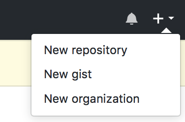
Click on “New repository” and then create a new repository like this:
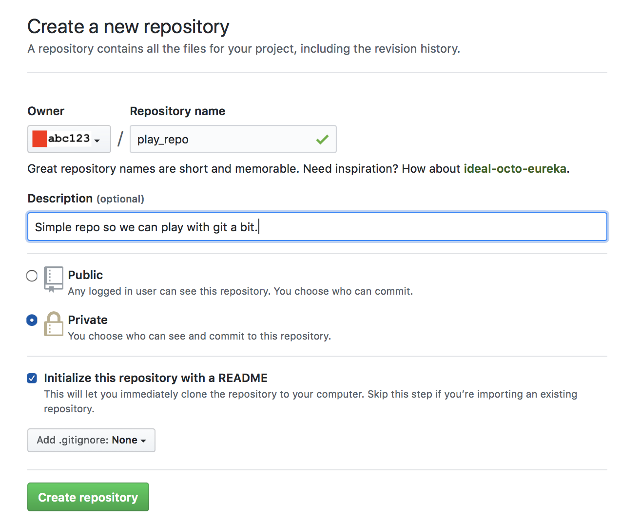
Note that the default setting is to make your repository public (visible to everyone). Any repository that contains code for this course should be made private; a public repository shares your code with others which constitutes an academic integrity violation.
Now click on the green “Create Repository” button.
Set Up Credentials
Before you can clone your repository (get a local copy to work on), you will need to set up SSH credentials with GitHub.
First, generate an SSH key if you don’t already have one. Just type this command:
ssh-keygen -C "<netid>@cornell.edu"
and use your NetID. The prompts will let you protect your key with a passphrase if you want.
Next, follow the instructions from GitHub to add the new SSH key to your GitHub account.
To summarize, go to Settings -> SSH and GPG Keys -> New SSH key,
and then paste the contents of a file named something like ~/.ssh/id_rsa.pub.
Clone the Repository
Cloning a git repository means that you create a local copy of its contents. You should clone the repository onto your own local machine (lab computer or laptop).
Find the green button on the right side of the GitHub webpage for your repository that says “Code”. Click it, then choose the “SSH” tab. Copy the URL there, which will look like this:
git@github.coecis.cornell.edu:abc123/play_repo.git
In a terminal, navigate to the folder where you would like to put your repository, and type:
git clone <PASTE>
That is, just type git clone (then a space) and paste the URL from GitHub.
Run this command to download the repository from GitHub to your computer.
At this point, you’ll get authentication errors if your SSH key isn’t set up correctly. So try that again if you get messages like “Please make sure you have the correct access rights and the repository exists.”
Look Around
Type cd play_repo to enter the repository. Type ls and you’ll see that your repo currently has just one file in it called README.md.
Type git status to see an overview of your repository. This command will show the status of your repository and the files that you have changed. At first, this command won’t show much.
Tracking Files with Git
There are 3 steps to track a file with git and send it to GitHub: stage, commit, and push.
Stage
To try it out, let’s make a new file.
Create a new file called <netid>.txt (use your NetID in there).
Now type git add NetID.txt from the directory containing the file to stage the file.
Staging informs git of the existence of the file so it can track its changes.
Type git status again.
You will see the file you added highlighted in green.
This means that the file is staged, but we still have two more steps to go to send your changes to GitHub.
(You might consider going back to the GitHub web interface to confirm that your new <netid>.txt file doesn’t show up there yet.)
Commit
A commit is a record of the state of the repository at a specific time. To make a commit, run this command:
git commit -m "Added my favorite color!"
The message after -m is a commit message, which is an explanation of the changes that you have made since you last committed. Good commit messages help you keep track of the work you’ve done.
This commit is now on your local computer. Try refreshing the GitHub repository page to confirm that it’s still not on the remote repository.
Push
To send our changes to the server, type this:
git push
The git push command sends any commits you have on your local machine to the remote machine.
You should imagine you are pushing them over the internet to GitHub’s servers.
Try refreshing the GitHub repository page again—now you should see your file there!
Pull
You will also want to retrieve changes from the remote server. This is especially helpful if you work on the repository from different machines. Type this command:
git pull
For now, this should just say that everything’s up to date. But if there were any new changes on the server, this would download them.
Typical Usage Pattern
Here is a good git workflow you should follow:
git pull: Type this before you start working to make sure you’re working on the most up to date version of your code (also in case the staff had to push any updates to you).- Work on your files.
git add file.txt: Type this for each file you either modified or added to the repo while you were working. Not sure what you touched or what’s new? Typegit statusand git will tell you!git commit -m "very helpful commit message": Save your changes in a commit. Write a message to remind your future self what you did.git push: Remember that, without the push, the changes are only your machine. If your laptop falls in a lake, then they’re gone forever. Push them to the server for safekeeping.
Git can be a little overwhelming, and sometimes the error messages can be hard to understand. Most of the time, following the instructions git gives you will help; if you run into real trouble, though, please ask a TA. If things get really messed up, don’t be afraid to clone a new copy of your repository and go from there.
It is completely OK to only know a few of the most common git commands and to not really understand how the whole thing works.
Many professional programmers get immense value out of git while only ever using add, commit, push, and pull.
Don’t worry about learning everything about git up front—you are already ready to use it productively!
Even More Commands
Here are a few other commands you might find useful. This is far from everything—there is a lot more in the git documentation.
Log
Type this command:
git log <netid>.txt
You’ll see the history of README.md.
You will see the author, time, and commit message for every commit of this file, along with the commit hash, which is how Git labels your commits and how you reference them if you need to.
At this point, you’ll only see a single commit.
But if you were to change the file and run git commit again, you would see the new change in the log.
You can also type git log with no filename afterward to get a history of all commits in your entire repository.
Stash
If you want to revert to the state of the last commit after making some new changes, you can type git stash.
Stashed changes are retrievable, but it might be a hassle to do so.
git stash only works on changes that have not yet been committed.
If you accidentally commit a change and want to wipe it out before pulling work from other machines, use git reset HEAD~1 to undo the last commit (and then stash).
Introduction to SSH
SSH (Secure SHell) is a tool that lets you connect to another computer over the Internet to run commands on it.
You run the ssh command in your terminal to use it.
The Cornell CS department has several machines available to you, if you want to use them to do your work. SSH is the (only) way to connect to these machines.
Accessing Cornell Resources from Off Campus
Cornell’s network requires you to be on campus to connect to Cornell machines. (This is a security measure: it is meant to prevents attacks from off campus.)
To access Cornell machines when you’re elsewhere, Cornell provides a mechanism called a Virtual Private Network (VPN) that lets you pretend to be on campus. Read more about Cornell’s VPN if you need it.
Log On
Make sure you are connected to the VPN or Cornell’s WiFi. Open a terminal window and type:
ssh <netid>@ugclinux.cs.cornell.edu
but replace <>).
Type yes and hit enter to accept the new SSH host key.
Now type your NetID password.
You’re in! You should see a shell prompt; you can follow the Unix shell tutorial to learn how to use it.
Here, ugclinux.cs.cornell.edu is the name of a collection of servers that Cornell runs for this purpose.
That’s what you’d replace with a different domain name to connect to a different machine.
scp
Suppose you have a file on the ugclinux machines and you want to get a copy locally onto your machine.
The scp command can do this.
It works like a super-powered version of the cp command that can copy between machines.
Say your file game.c is located at /home/yourNetID/mygame/game.c on ugclinux.
On your local machine (i.e., when not connected over SSH already), type:
scp yourNetID@ugclinux.cs.cornell.edu:mygame/game.c .
Here are the parts of that command:
scp <user>@<host>:<source> <dest>
<user> and <host> are the same information you use to connect to the remote machine with the ssh command.
<source> is the file on that remote machine that you want to obtain,
and <dest> is the place where you want to copy that file to.
Makefile Basics
This document is meant to serve as a very brief reference on how to read the Makefiles provided in this class. This tutorial is meant to be just enough to help you read the Makefiles you provide, and is not meant to be a complete overview of Makefiles or enough to help you make your own. If you are interested in learning more, there are some good tutorials online, such as this walkthrough.
A Makefile is often used with C to help with automating the (repetitive) task of compiling multiple files. This is especially helpful in cases where there are multiple pieces of your codebase you want to compile separately, such as choosing to test a program or run that program.
Variables
To illustrate how this works, let us examine a few lines in the Makefile that will be used for the minifloat assignment. Our first line of code is to define a variable CFLAGS:
CFLAGS=-Wall -Wpedantic -Werror -Wshadow -Wformat=2 -Wconversion -std=c99
As in other settings, defining this variable CFLAGS allows us to use the contents (a string in this case) later in our Makefile. Our specific choice of CFLAGS here is to indicate that we are defining the flags (for C) that we will be using in this Makefile. Later, when we use this variable in-line, the Makefile will simply replace the variable with whatever we defined it as, thus allowing us to use the same flags consistently for every command we run.
Commands
The rest of our Makefile for this assignment will consist of commands. A command has the following structure:
name: dependent_files
  operation_to_run
The name of a command is what you run in your terminal after make, such as make part1 or make all (this gets a bit more complicated in some cases). The dependent_files indicate which files this command depends on – the Makefile will only run this command if one of these files changed since the last time we ran it. Finally, the operation is what actually gets run in our console, such as when we run gcc main.c -o main.o.
Example Command
To make this more concrete, let us examine our first command for part1:
part1: minifloat.c minifloat_test_part1.c minifloat_test_part1.expected
	$(CC) $(CFLAGS) minifloat.c minifloat_test_part1.c -o minifloat_test_part1.out
This command will execute when we run make part1, but only if one of minifloat.c, minifloat_test_part1.c or minifloat_test_part1.expected have been modified since we last ran this command. What actually runs is the next line, with the $(CC), $(CFLAGS), and a bunch of filenames. $(CC) is a standard Makefile variable that is replaced by our C compiler – in our case, this is gcc. The $(CFLAGS) variable here is what we defined earlier, so we include all of the flags we desired. Finally, the list of files is exactly the same as we might normally run with gcc. In total, then, this entire operation will be translated to:
$(CC) $(CFLAGS) minifloat.c minifloat_test_part1.c -o minifloat_test_part1.out
-->
gcc $(CFLAGS) minifloat.c minifloat_test_part1.c -o minifloat_test_part1.out
-->
gcc -Wall -Wpedantic -Werror -Wshadow -Wformat=2 -Wconversion -std=c99 minifloat.c minifloat_test_part1.c -o minifloat_test_part1.out
This compilation would be a huge pain to type out everytime, especially with all of those flags (and easy to mess up), but with the Makefile, we can run all this with just make part1. We can do the same with make part2 to run the next set of commands instead.
Clean
One final node is that it is conventional (though not required) to include a make clean that removes any generated files, often for being able to clean up our folder or push our work to a Git repository. In our particular file, we have defined clean to remove the generated .out files and any .txt files that were used for testing:
clean:
	rm -f *.out.stackdump
	rm -f *.out
	rm -f *.txt
Complete Makefile
For reference, the entirity of our Makefile is included here:
CFLAGS=-Wall -Wpedantic -Werror -Wshadow -Wformat=2 -Wconversion -std=c99
CC = gcc

all: part1 part2 part3

part1: minifloat.c minifloat_test_part1.c minifloat_test_part1.expected
	$(CC) $(CFLAGS) minifloat.c minifloat_test_part1.c -o minifloat_test_part1.out

part2: minifloat.c minifloat_test_part2.c
	$(CC) $(CFLAGS) minifloat.c minifloat_test_part2.c -o minifloat_test_part2.out

part3: minifloat.c minifloat_test_part3.c
	$(CC) $(CFLAGS) minifloat.c minifloat_test_part3.c -o minifloat_test_part3.out

clean:
	rm -f *.out.stackdump
	rm -f *.out
	rm -f *.txt

.PHONY: all clean
C Programming
Much of the work in CS 3410 involves programming in C. This section of the site contains some overviews of most of the C features you will need in CS 3410.
For authoritative details on C and its standard library,
the C reference on cppreference.com (despite the name) is a good place to look.
For example, here’s a list of all the functions in the stdio.h header, and here’s the documentation specifically about the fputs function.
Compiling and Running C Code
Before you proceed with this page, follow the instructions to set up the course’s RISC-V infrastructure.
Your First C Program
Copy and paste this program into a text file called first.c:
#include <stdio.h>

int main() {
    printf("Hello, CS 3410!\n");
    return 0;
}
Next, run this command:
rv gcc -o first first.c
Here are some things to keep in mind whenever these pages ask you to run a command:
- Our course’s RISC-V infrastructure setup has you create an
rvalias for running commands inside the infrastructure container. We will not always include anrvprefix on example commands we list in these pages. Whenever you need to run a tool that comes from the container, use thervprefix or some other mechanism to make sure the command runs in the container. - As with all shell commands, it really matters which directory you’re currently “standing in,” called the working directory. Here,
first.candfirstare both filenames that implicitly refer to files within the working directory. So before running this command, be sure tocdto the place where yourfirst.cfile exists.
If everything worked, you can now run this program with this command:
rv qemu first
Your output should look like this:
Hello, CS 3410!
This command uses QEMU, an emulator for the RISC-V instruction set, to run the program we just compiled, which is in the file named first.
Recommended Options
While the simple command gcc -o first first.c works fine for this simple example, we officially recommend that you always use a few additional command-line options that make the GCC compiler more helpful.
Here are the ones we recommend:
-Wall -Wextra -Wpedantic -Wshadow -Wformat=2 -std=c23
In other words, here’s our complete recommended command for compiling your C code:
rv gcc -Wall -Wextra -Wpedantic -Wshadow -Wformat=2 -std=c23 hi.c
Many assignments will include a Makefile that supplies these options for you.
Checking for Common C Errors
Memory-related bugs in C programs are extremely common! The worst thing about them is that they can cause obscure problems silently, without even crashing with a reasonable error message. Fortunately, GCC has built-in tools called sanitizers that can (much of the time, but not always) catch these bugs and give you reasonable error messages.
To use the sanitizers, add these flags to your compiler command:
-g -fsanitize=address -fsanitize=undefined
So here’s a complete compiler command with sanitizers enabled:
rv gcc -Wall -Wextra -Wpedantic -Wshadow -Wformat=2 -std=c23 -g -fsanitize=address -fsanitize=undefined hi.c
Then run the resulting program to check for errors.
Unfortunately, LeakSanitizer, the part of AddressSanitizer that detects memory leaks, does not work properly on RISC-V platforms. As a result, memory leaks will not be caught when using the sanitizers within our infrastructure container.
Instead, we will attempt to provide leak check smoke tests on Gradescope which check for memory leaks when you submit your code.
We recommend trying the sanitizers whenever your code does something mysterious or unpredictable. It’s an unfortunate fact of life that, unlike many other languages, bugs in C code can silently cause weird behavior; sanitizers can help counteract this deeply frustrating problem.
C Basics
This section is an overview of the basic constructs in any C program.
Variable Declarations
C is a statically typed languages, so when you declare a variable, you must also declare its type.
int x;
int y;
Variable declarations contain the type (int in this example) and the variable name (x and y in this example).
Like every statement in C, they end with a semicolon.
Assignment
Use = to assign new values to variables:
int x;
x = 4;
As a shorthand, you can also include the assignment in the same statement as the declaration:
int y = 6;
Expressions
An expression is a part of the code that evaluates to a value, like 10 or 7 * (4 + 2) or 3 - x.
Expressions appear in many places, including on the right-hand side of an = in an assignment.
Here are a few examples:
int x;
x = 4 + 3 * 2;
int y = x - 6;
x = x * y;
Functions
To define a function, you need to write these things, in order: the return type, the function name, the parameter list (each with a type and a name), and then the body. The syntax looks like this:
<return type> <name>(<parameter type> <parameter name>, ...) {
    <body>
}
Here’s an example:
int myfunc(int x, int y) {
  int z = x - 2 * y;
  return z * x;
}
Function calls look like many other languages:
you write the function name and then, in parentheses, the arguments.
For example, you can call the function above using an expression like myfunc(10, 4).
The main Function
Complete programs must have a main function, which is the first one that will get called when the program starts up.
main should always have a return type of int.
It can optionally have arguments for command-line arguments (covered later).
Here’s a complete program:
int myfunc(int x, int y) {
  int z = x - 2 * y;
  return z * x;
}

int main() {
  int z = myfunc(1, 2);
  return 0;
}
The return value for main is the program’s exit status.
As a convention, an exit status of 0 means “success” and any nonzero number means some kind of exceptional condition.
So, most of the time, use return 0 in your main.
Includes
To use functions declared somewhere else, including in the standard library, C uses include directives. They look like this:
#include <hello.h>
#include "goodbye.h"
In either form, we’re supplying the filename of a header file.
Header files contain declarations for functions and variables that C programs can use.
The standard filename extension for header files in C is .h.
You should use the angle-bracket version for library headers and the quotation-mark version for header files you write yourself.
Printing
To print output to the console, use printf, a function from the C standard library which takes:
- A string to print out, which may include format specifiers (more on these in a moment).
- For each format specifier, a value to fill in for each format specifier.
The first string might have no format specifiers at all, in which case the printf only has a single argument.
Here’s what that looks like:
#include <stdio.h>

int main() {
  printf("Hello, world!\n");
}
The \n part is an escape sequence that indicates a newline, i.e., it makes sure the next thing we output goes on the next line.
Format specifiers start with a % sign and include a few more characters describing how to print each additional argument.
For example, %d prints a given argument as a decimal integer.
Here’s an example:
#include <stdio.h>

int main() {
  int x = 3;
  int y = 4;
  printf("x + y = %d.\n", x + y);
}
Here are some format specifiers for printing integers in different bases:
| Base | Format Specifier | Example |
|---|---|---|
| decimal | %d | printf("%d", i); |
| hexadecimal | %x | printf("%x", i); |
| octal | %o | printf("%o", i); |
And here are some common format specifiers for other data types:
| Data Type | Format Specifier | Example |
|---|---|---|
string | %s | printf("%s", str); |
char | %c | printf("%c", c); |
float | %f | printf("%f", f); |
double | %lf | printf("%lf", d); |
long | %ld | printf("%ld", l); |
long long | %lld | printf("%lld", ll); |
| pointers | %p | printf("%p", ptr); |
See the C reference for details on the full set of available format specifiers.
Basic Types in C
Some Common Data Types
| Type | Common Size in Bytes | Interpretation |
|---|---|---|
char | 1 | one ASCII character |
int | 4 | signed integer |
float | 4 | single-precision floating-point number |
double | 8 | double-precision floating-point number |
A surprising quirk about C is that the sizes of some types can be different in different compilers and platforms! So this table lists common byte sizes for these types on popular platforms.
Characters
Every character is corresponds to a number. The mapping between characters and numbers is called the text encoding, and the ubiquitous one for basic characters in the English language is called ASCII. Here is a table with some of the most common characters in ASCII:
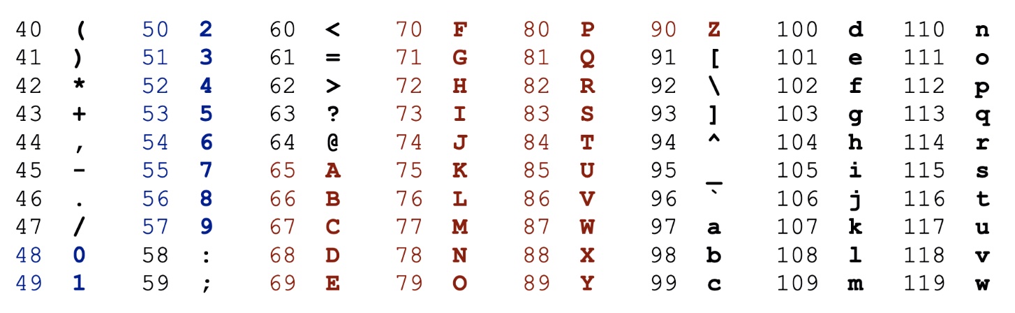
For all the characters in ASCII (and beyond), see this ASCII table.
Booleans
C does not have a bool data type available by default.
Instead, you need to include the stdbool.h header:
#include <stdbool.h>
That lets you use the bool type and the true and false expressions.
If you get an error like unknown type name 'bool', just add the include above to fix it.
Prototypes and Headers
Declare Before Use
In C, the order of declarations matters. This program with two functions works fine:
#include <stdio.h>

void greet(const char* name) {
  printf("Hello, %s!\n", name);
}

int main() {
  greet("Eva");
  return 0;
}
But what happens if you just reverse the two function definitions?
#include <stdio.h>

int main() {
  greet("Eva");
  return 0;
}

void greet(const char* name) {
  printf("Hello, %s!\n", name);
}
The compiler gives us this somewhat confusing error message:
error: implicit declaration of function 'greet'
The problem is that, in C,
you have to declare every name before you can use it.
So the declaration of greet has to come earlier in the file than the call to greet("Eva").
Declarations, a.k.a. Prototypes
This declare-before-use rule can make it awkward to define functions in the order you want, and it seems to be a big problem for mutual recursion. Fortunately, C has a mechanism to let you declare a name before you define what it means. All the functions we’ve seen so far have been definitions (a.k.a. implementations), because they include the body of the function. A function declaration (a.k.a. prototype) looks the same, except that we leave off the body and just write a semicolon instead:
void greet(const char* name);
A declaration like this tells the compiler the name and type of the function, and it amounts to a promise that you will later provide a complete definition.
Here’s a version of our program above that works and keeps the function definition order we want (main and then greet):
#include <stdio.h>

void greet(const char* name);

int main() {
  greet("Eva");
  return 0;
}

void greet(const char* name) {
  printf("Hello, %s!\n", name);
}
By including the declaration at the top of the file, we are now free to call greet even though the definition comes later.
Header Files
It is so common to need to declare a bunch of functions so you can call them later that C has an entire mechanism to facilitate this:
header files.
A header is a C source-code file that contains declarations that are meant to be included in other C files.
You can then “copy and paste” the contents of header files into other C code using the #include directive.
Even though the C language makes no formal distinction between what you can do in headers and in other files, it is a universal convention that headers have the .h filename extension while “implementation” files use the .c extension.
For example, we could put our greet declaration into a utils.h header file:
void greet(const char* name);
Then, we might put this in main.c:
#include <stdio.h>
#include "utils.h"

int main() {
  greet("Eva");
  return 0;
}

void greet(const char* name) {
  printf("Hello, %s!\n", name);
}
The line #include "utils.h" instructs the C preprocessor to look for the file called utils.h and paste its entire contents in at that location.
Because the preprocessor runs before the compiler, this two-file version of our project looks exactly the same to the compiler as if we had merged the two files by hand.
You can read more about #include directives, including about the distinction between angle brackets and quotation marks.
Multiple Source Files
Eventually, your C programs will grow large enough that it’s inconvenient to keep them in one .c file.
You could distribute the contents across several files and then #include them, but there is a better way:
we can compile source files separately and then link them.
To make this work in our example, we will have three files.
First, our header file utils.h, as before, just contains a declaration:
void greet(const char* name);
Next, we’re write an accompanying implementation file, utils.c:
#include <stdio.h>
#include "utils.h"

void greet(const char* name) {
  printf("Hello, %s!\n", name);
}
As a convention, C programmers typically write their programs as pairs of files:
a header and an implementation file, with the same base name and different extensions (.h and .c).
The idea is that the header declares exactly the set of functions that the implementation file defines.
So in that way, the header file acts as a short “table of contents” for what exists in the longer implementation file.
Let’s call the final file main.c:
#include "utils.h"

int main() {
  greet("Eva");
  return 0;
}
Notably, we use #include "utils.h" to “paste in” the declaration of greet, but we don’t have its definition here.
Now, it’s time to compile the two source files, utils.c and main.c.
Here are the commands to do that:
gcc -c utils.c -o utils.o
gcc -c main.c -o main.o
(Remember to prefix these commands with rv to use our RISC-V infrastructure.)
The -c flag tells the C compiler to just compile the single source file into an object file, not an executable.
An object file contains all code for a single C source program, but it is not directly runnable yet—for one thing, it might not have a main function.
Using -o utils.o tells the compiler to put the output in a file called utils.o.
As a convention, the filename extension for object files is .o.
You’ll notice that we only compiled the .c files, not the .h files.
This is intentional: header files are only for #includeing into other files.
Only the actual implementation files get compiled.
Finally, we need to combine the two object files into an executable. This step is called linking. Here’s how to do that:
gcc utils.o main.o -o greeting
We supply the compiler with two object files as input and tell it where to put the resulting executable with -o greeting.
Now you can run the program:
./greeting
(Use rv qemu greeting to use the course RISC-V infrastructure.)
Control Flow
Logical Operators
Here are some logical operators you can use in expressions:
| Expression | True If… |
|---|---|
expr1 == expr2 | expr1 is equal to expr2 |
expr1 != expr2 | expr1 is not equal to expr2 |
expr1 < expr2 | expr1 is less than expr2 |
expr1 <= expr2 | expr1 is less than or equal to expr2 |
expr1 > expr2 | expr1 is greater than expr2 |
expr1 >= expr2 | expr1 is greater than or equal to expr2 |
!expr | expr is false (i.e., zero) |
expr1 && expr2 | expr1 and expr2 are true |
expr1 || expr2 | expr1 or expr2 is true |
false && expr2 will always evaluate to false, and true || expr2 will always evaluate to true, regardless of what expr2 evaluates to.
This is called “short circuiting”: C evaluates the left-hand side of these expressions first and, if the truth value of that expression means that the other one doesn’t matter, it won’t evaluate the right-hand side at all.
Conditionals
Here is the syntax for if/else conditions:
if (condition) {
  // code to execute if condition is true
} else if (another_condition) {
  // code to execute if condition is false but another_condition is true
} else {
  // code to execute otherwise
}
The else if and else parts are optional.
Switch/Case
A switch statement can be a succinct alternative to a cascade of if/elses when you are checking several possibilities for one expression.
switch (expression) {
  case constant1:
    // code to execute if expression equals constant1
    break;
  case constant2:
    // code to execute if expression equals constant2
    break;
  // ...
  default:
    // code to be executed if expression doesn't match any case
}
While Loop
while (condition) {
  // code to execute as long as condition is true
}
For Loop
for (initialization; condition; increment) {
  // code to execute for each iteration
}
Roughly speaking, this for loop behaves the same way as this while equivalent:
initialization;
while (condition) {
  // code to execute for each iteration
  increment;
}
break and continue
To exit a loop early, use a break; statement.
A break statement jumps out of the innermost enclosing loop or switch statement.
If the break statement is inside nested contexts, then it exits only the most immediately enclosing one.
To skip the rest of a single iteration of a loop, but not cancel the loop entirely, use continue.
Declaring Your Own Types in C
Structures
The struct keyword lets you declare a type that bundles together several values, possibly of different types.
To access the fields inside a struct variable, use dot syntax, like thing.field.
Here’s an example:
struct rect_t {
  int left;
  int bottom;
  int right;
  int top;
};

int main() {
  struct rect_t myRect;
  myRect.left = -4;
  myRect.bottom = 1;
  myRect.right = 8;
  myRect.top = 6;

  printf("Bottom left = (%d,%d)\n", myRect.left, myRect.bottom);
  printf("Top right = (%d,%d)\n", myRect.right, myRect.top);

  return 0;
}
This program declares a type struct rect_t and then uses a variable myRect of that type.
Enumerations
The enum keyword declares a type that can be one of several options.
Here’s an example:
enum threat_level_t {
  LOW,
  GUARDED,
  ELEVATED,
  HIGH,
  SEVERE
};

void printOneLevel(enum threat_level_t threat) {
  switch (threat) {
    case LOW:
      printf("Green/Low.\n");
      break;
    // ...omitted for brevity...
    case SEVERE:
      printf("Red/Severe.\n");
      break;
  }
}

void printLevels() {
  printf("Threat levels are:\n");
  for (int i = LOW; i <= SEVERE; i++) {
    printOneLevel(i);
  }
}
This code declares a type enum threat_level_t that can be one of 5 values.
Type Aliases
You can use the typedef keyword to give new names to existing types.
Use typedef <old type> <new name>;, like this:
typedef int whole_number;
Now, you can use whole_number to mean the same thing as int.
Short Names for Structs and Enums
You may have noticed that struct and enum declarations make types that are kind of long and hard to type.
For example, we declared a type enum threat_level_t.
Wouldn’t it be nice if this type could just be called threat_level_t?
typedef is also useful for defining these short names.
You could do this:
enum _threat_level_t { ... }
typedef enum _threat_level_t threat_level_t;
And that does work! But there’s also a shorter way to do it, by combining the enum and the typedef together:
typedef enum {
  ...
} threat_level_t;
That defines an anonymous enumeration and then immediately gives it a sensible name with typedef.
Below is a helpful table which summarizes the different ways that you can
declare and initialize a struct (or an enum).
| Description | Declaration | Declaration & Initialization |
|---|---|---|
Define a type struct rect_t only.
|
|
myRect has type struct rect_t
|
Define a type struct _rect_t and then define its type alias rect_t.
|
|
|
Define a type struct _rect_t and its type alias rect_t in the same statement.
|
|
|
Define a type rect_t.
|
|
|
Bit Packing
Structs work well when you want to combine several types that have “nice” sizes: 1, 4, or 8 bytes, for example.
But they can waste space if you actually only need a few bits for your values.
For example, we learned that the float type is 32 bits: 1 sign bit, 8 exponent bits, and 23 significand bits.
If we wanted to “fake” a floating-point number with a struct, we couldn’t use a 1-bit and 23-bit type.
The best we can do is to use 8 bits, 8 bits, and 32 bits:
#include <stdio.h>
#include <stdint.h>

typedef struct {
    uint8_t sign;
    uint8_t exponent;
    uint32_t significand;
} fake_float_t;

int main() {
    printf("size: %lu\n", sizeof(fake_float_t));
}
That struct uses a total of 6 bytes for its fields.
But compilers often need to insert padding to make sure values are aligned for efficient memory access, so the struct can be bigger than that.
Here, we use sizeof to measure the actual total size of the struct, which is 8 bytes—twice as big as a real 4-byte float!
This section will show you how to pack these irregularly-sized values into integers—a trick that you can call bit packing.
The big idea is to treat integer types like uint32_t just as sequences of bits rather than as actual integers, and to use C’s built-in bit-manipulation operations to insert and extract ranges of bits.
The key operations are:
- Masking, with the bitwise “and” operator,
&. - Combining, with the bitwise “or” operator,
|. - Shifting, with the bitwise shift operators
>>and<<.
You may find it helpful to look over the full list of arithmetic and bit manipulation operators in C.
Shifting
In C, i << n shifts the bits in an integer i leftward by n places,
filling in the bottom n bits with zeroes.
Mathematically, this has the effect of multiplying i by \(2^n\):
#include <stdio.h>
#include <stdint.h>

int main() {
    uint32_t n = 21;
    printf("double n: %u\n", n << 1);
}
Similarly, i >> n shifts the bits rightward by n places, so it multiplies i by \(2^{-n}\).
These shift operations are useful for moving bit patterns around within the range of bits in the value.
Let’s try moving a value around in a uint32_t and printing out the bits:
#include <stdio.h>
#include <stdint.h>

int main() {
    uint32_t n = 21;
    printf("%032b\n", n);
    printf("%032b\n", n << 8);
    printf("%032b\n", n << 16);
    printf("%032b\n", n << 24);
}
That %032b specifier tells printf to pad the value out to 32 bits for consistency.
If you run this program, you can see the bit-pattern for the value 21 moving around within the range of 32 bits:
00000000000000000000000000010101
00000000000000000001010100000000
00000000000101010000000000000000
00010101000000000000000000000000
Combining
The bitwise “or” operator, written in C with a single |, is useful for combining different values that have been shifted to different places.
The insight is that x | 0 == x for any bit x, and our shifted values have zeroes wherever they are “inactive.”
Let’s try shifting two different small values to two different positions and then combining them:
#include <stdio.h>
#include <stdint.h>

int main() {
    uint32_t x = 21;
    uint32_t y = 17;
    printf("x:      %032b\n", x);
    printf("y<<8:   %032b\n", y << 8);
    printf("x|y<<8: %032b\n", x | (y << 8));
}
If you run this program, you can see the bit patterns for 21 and 17 coexisting happily, side-by-side. Because we know these values fit in 8 bits, we can think of the first value occupying bits 0 through 7 (numbered from the least significant bit) and the next one occupying bits 8 through 15 in the combined value.
Masking
Next, we want a way to extract bits out of one of these combined values.
The idea is to use the bitwise “and” operator, &, together with a mask value that has ones exactly where the bits are that we’re interested in.
We’ll use this property of the & operator:
- Wherever
maskis 1,mask & x == xfor any bitx. - Wherever
maskis 0,mask & x == 0for any bit0.
So a mask value has the effect of preserving values from x where it’s 1 and ignoring them (turning them into to 0) where it’s 0.
Let’s construct a mask to separate the two packed values from last time:
#include <stdio.h>
#include <stdint.h>

int main() {
    uint32_t x = 21;
    uint32_t y = 17;
    uint32_t comb = x | (y << 8);
    printf("comb:        %032b\n", comb);

    uint32_t x_mask = 0b00000000000000000000000011111111;
    uint32_t y_mask = 0b00000000000000001111111100000000;

    printf("comb&x_mask: %032b\n", comb & x_mask);
    printf("comb&y_mask: %032b\n", comb & y_mask);
}
Running this program will show how we’ve “separated” the combined value back into its constituent parts.
When writing masks, it can get really tiresome to write all those ones and zeroes out.
It’s often more practical to write them as hexadecimal literals, remembering that every hex digit corresponds to 4 bits (a nibble):
hex 0 is binary 0000,
and hex F is binary 1111.
So this program is equivalent:
#include <stdio.h>
#include <stdint.h>

int main() {
    uint32_t x = 21;
    uint32_t y = 17;
    uint32_t comb = x | (y << 8);
    printf("comb:        %032b\n", comb);

    uint32_t x_mask = 0x000000FF;
    uint32_t y_mask = 0x0000FF00;

    printf("comb&x_mask: %032b\n", comb & x_mask);
    printf("comb&y_mask: %032b\n", comb & y_mask);
}
Putting it All Together
Now that we’ve separated the two values out by masking the combined value, there is one more step to recover the original values.
We just need to shift them right with >> back to their original positions.
Actually, x is already in its original position, so we don’t have to do anything to it.
But y was shifted left by 8 bits originally, so to get its original value, we’ll shift the masked-out value right again by the same amount.
Here’s a complete program that shows the combination and extraction together:
#include <stdio.h>
#include <stdint.h>

uint32_t pack(uint8_t x, uint8_t y) {
    return x | (y << 8);
}

uint8_t get_x(uint32_t comb) {
    return comb & 0x000000FF;
}

uint8_t get_y(uint32_t comb) {
    return (comb & 0x0000FF00) >> 8;
}

int main() {
    uint32_t comb = pack(34, 10);
    printf("recovered x: %hhd\n", get_x(comb));
    printf("recovered y: %hhd\n", get_y(comb));
}
The pack function combines x and y into a single uint32_t.
Then, the get_x and get_y functions use masking and shifting to undo this combination and extract the original values.
Bit packing is a superpower that you have unlocked by understanding how values are represented at the level of bits.
Use it to save space when ordinary structs won’t cut it!
Pointers!
Pointers are central to programming in C, yet are often one of the most foreign concepts to new C coders.
A Motivating Example
Suppose we want to write a swap function that will take two integers and swap their values. With the programming tools we have so far, our function might look something like this:
void swap(int a, int b) {
  int temp = a;
  a = b;
  b = temp;
}
This won’t work how we want it to!
If we call swap(foo, bar), the swap function gets copies of the values in foo and bar.
Reassigning a and b just affects those copies—not foo and bar
themselves! (This behavior is called call by value (or pass by value) as the values of
the variables are passed as function arguments, not references.)
How can we give swap direct access to the places where the arguments are stored so it can actually swap them?
Pointers are the answer.
Pointers are addresses in memory, and you can think of them as referring to a value that lives somewhere else.
Declaring a Pointer
For any type T, the type of a pointer to a value of that type is T*: that is, the same type with a star after it.
For example, this code:
char* my_char_pointer;
(pronounced “char star my char pointer”) declares a variable with the name my_char_pointer.
This variable is not a char itself!
Instead, it is a pointer to a char.
Confusingly, the spaces don’t matter. The following three lines of code are all equivalent declarations of a pointer to an integer:
int* ptr;
int *ptr;
int * ptr;
ptr has the type “pointer to an integer.”
Initializing a Pointer
int* ptr = NULL;
The line above initializes the pointer to NULL, or zero. It means the pointer does not point to anything. This is a good idea if you don’t plan on having it point to something just yet. Initializing to NULL helps you avoid “dangling” pointers which can point to random memory locations that you wouldn’t want to access unintentionally. C will not do this for you.
You can check if a pointer is NULL with the expression ptr == NULL.
The current C programming language standard, C23, introduces a new nullptr
keyword which denotes a null pointer constant. The type of nullptr is also
new, the aptly named nullptr_t. In fact, nullptr is the only valid value
of type nullptr_t.
For compatibility with older C language standards, we recommend still using
NULL to check for null pointers, even though in most cases. Indeed, it is
likely that on your machine NULL is defined to be nullptr!
Assigning to a Pointer, and Getting Addresses
In the case of a pointer, changing its value means changing where it points. For example:
void func(int* x) {
  int* y = x;
  // ...
The assignment in that code makes y and x point to the same place.
But what if you want to point to a variable that already exists?
C has an & operator, called the “address-of” (or “reference-of”) operator, that gets the pointer to a variable.
For example:
int x = 5;
int* xPtr = &x;
Here, xPtr now points to x.
You can’t assign to the address of things; you can only use & in expressions (e.g., on the right-hand side of an assignment).
So:
y = &x;  // this is fine
&x = y;  // will not compile!
This rule reflects the fact that you can get the location of any variable, but it is never possible to change the location of a variable.
Dereferencing Pointers
Once you have a pointer with a memory location in it, you will want to access the value that is being pointed at—either reading or changing the value in the box at the end of the arrow.
For this, C has the * operator, known as the “dereference” operator because it follows a reference (pointer) and gives you the referred-to value.
You can both read from and write to a dereferenced pointer, so * expressions can appear on either side of an assignment.
For example:
int number = *xPtr;  // read the value xPtr points to
printf("the number is %d\n", *xPtr);  // read it and then print it
*xPtr = 6;  // write the value that xPtr points to
Common Confusion with the * Operator
Do not be confused by the two contexts in which you will see the star (*) symbol:
- Declaring a pointer:
int* p; - Dereferencing a pointer (RHS):
r = *p; - Dereferencing a pointer (LHS):
*p = r;
The star is part of the type name when declaring a pointer and is the dereference operator when used in assignments.
Swap with Pointers
Now that we have pointers, we can correctly write that swap function we wanted! The new version of swap uses a “pass by reference” model in which pointers to arguments are passed to the function.
void swap(int* a, int* b) {
  int temp = *a;
  *a = *b;
  *b = temp;
}
The Arrow Operator
Recall that we used the “dot” operator to access elements within a struct, like myRect.left.
If you instead have a pointer to a struct, you need to dereference it first before you can access its fields,
like (*myRect).left.
Fortunately, C has a shorthand for this case!
You can also write myRect->left to mean the same thing.
In other words, the -> operator works like the . operator except that it also dereferences the pointer on the left-hand side.
Pointer Arithmetic
If pointers are just addresses in memory, and addresses are just integers,
you might wonder if you can do arithmetic on them like you can with ints.
Yes, you can!
Adding n to a pointer to any type T causes the pointer to point n Ts further in memory.
For example, the expression ptr + offset might compute a pointer that is “four ints later in memory” or “six chars later in memory.”
int x = 5;
int *ptr = ...;

x = x + 1;
ptr = ptr + 1;
In this code:
x + 1: adds 1 to to the integerx, producing 6ptr + 1: adds the size of anintin bytes toptr, shifting to point to the next integer in memory
Printing Pointers
You can print the address of a pointer to see what memory location it is pointing to. For example:
printf("Pointer address: %p\n", (void*)ptr);
This will output the memory address the pointer ptr is currently holding.
Arrays
An array is a sequence of same-type values that are consecutive in memory.
Declaring an Array
To declare an array, specify its type and size (i.e., the number of items in the sequence). For example, an array of four integers can be declared as follows:
int myArray[4];
A few variations on this declaration are:
int myArray[4] = {42, 45, 65, -5}; // initializes the values in the array
int myArray[4] = {0};              // initializes all the values in the array to 0
int myArray[] = {42, 45, 65, -5};  // initializes the values in the array, compiler intuits the array size
Accessing an Array
To refer to an element, specify the array name (e.g., my_array) and the position number (e.g., 0):
// Declare an array of five `int`s called `my_array`.
int my_array[5];
// Store the integer `8` at position `0` in array `my_array`.
my_array[0] = 8;
printf("I just initialized the element at index 0 to %d!\n", my_array[0]);
After executing the above code, my_array would look like this in memory (where
larger addresses are higher on the screen):
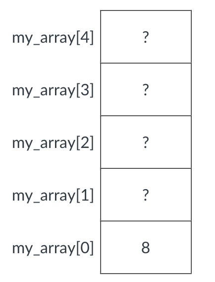
Ex: Compute the sum an array
To sum the elements of an array, we can use a for loop to iterate
over the array’s indices, adding the elements together as we go:
int sum_array(int *array, int n) {
  int sum = 0;
  for (int i = 0; i < n; ++i) {
    answer += array[i];
  }
  return sum;
}

int main() {
  int data[4] = {4, 6, 3, 8};
  int sum = sum_array(data, 4);
  printf("sum: %d\n", sum);
  return 0;
}
Accessing an Array using Pointer Arithmetic
In C, you can treat arrays as pointers: namely, to the first element in the sequence.
This means that, perhaps surprisingly, the syntax array[i] is shorthand for *(array + i):
that is, a combination of pointer arithmetic and dereferencing.
So you can think of array[i] as treating array as a pointer to the first element, then shifting the pointer over by i slots, and then dereferencing the pointer to that shifted location.
Passing Arrays as Parameters
You can also treat arrays as pointers when you pass them into functions. You already saw this above; we declared a function this way:
int sum_array(int *array, int n) { ... }
and then called it like sum_array(data, 4).
Even though we declared data as an array, C lets you treat it as a pointer to the first element.
C does not know the size of an array. As with many things in C, the language entrusts the programmer (i.e., you!) with that responsibility.
The rule of thumb is to pass around the length of the array in a separate parameter whenever you pass them into functions so you know how big the array is!
Common Pitfalls
- C has no array-bound checks. You won’t even get a warning! If you write past the end of an array, you will simply start overwriting the values of other data in memory.
sizeof(array)will return a different value based on how the variablearraywas declared. Ifarrayis declared asint *array, thenarraywill be considered the size of a pointer. If it was declared asint array[100]then it will be considered the size of 100ints.
Multidimensional Arrays
C lets you declare multidimensional arrays, like int matrix[4][3].
However, it still lays everything out sequentially in memory.
Here’s a visualization of what that matrix looks like conceptually and in memory:

This array occupies (4 * 3 * sizeof(double)) bytes of memory.
Strings
A string is an array of characters (chars), terminated by the null terminator character, '\0'.
In general, the type of a string in C is char*.
String Literals
We have seen string literals so far—a sequence of characters written down in quotation marks, such as "Hello World\n".
The type of a string literal is const char*, so this is valid C:
const char* str = "Hello World\n";
The const shows up here because the characters in a string literal cannot be modified.
Mutable Strings
A mutable string has type char*, without the const.
How can you declare a mutable string with a string literal, if string literals are always const?
Here’s a trick you can use:
remember that, in C, an array is like a pointer to its first element.
So let’s declare the string as an array and give it an initializer:
char str[] = "Hello World\n";
This code behaves exactly as if we wrote:
char str[] = {'H', 'e', 'l', 'l', 'o', ' ', 'W', 'o', 'r', 'l', 'd', '\n', '\0'};
It declares a variable str which is an array of 13 characters (remember that the size of an array may be implicit if we provide an initializer from which the compiler can determine the size), and initializes it by copying the characters of the string "Hello World\n" (including the null terminator) into that array.
String Equality
The expression str1 == str2 doesn’t check whether str1 and str2 are the same string!
Remember, since both of these have a pointer type (char*), C will just compare the pointers.
Instead, if you want to check whether two strings contain equal contents, you will need to use a function like strcmp from the string.h header.
String Copying
Similarly, an assignment like str1 = str2; does not copy strings!
It just just does pointer assignment, so now str1 points to the same region of memory as str2.
Use a function like strcpy if you need to copy characters.
C Macros
Let’s say you have a program that works with arrays of a certain size: say, 100 elements. The number 100 will show up in different parts of the code:
float stuff[100];

// ... elsewhere ...

for (int i = 0; i < 100; ++i) {
  do_something(stuff[i]);
}
Repeating the number 100 in multiple locations is not great for multiple reasons:
- It is not maintainable. If you ever need to change the size of the array, you need to carefully look for all the places where you mentioned 100 and change it to something else. If you happen to miss one, subtle bugs will arise.
- It is not readable. Writing code is as much about communicating with other programmers as it is about communicating with the machine! When a human sees the number 100 appear out of nowhere, it can be mysterious and worrisome. For this reason, programmers often call these arbitrary-seeming constants magic numbers (in a derogatory way).
C has a feature called the preprocessor that can cut down on duplication, eliminate magic numbers, and make code more readable. In particular, you can use a macro definition to give your constant a name:
#define NUMBER_OF_THINGS 100
The syntax #define <macro> <expression> defines a new name, the macro, and instructs the preprocessor to replace that name with the given expression.
(Notably, there is no semicolon after preprocessor directives like #define.)
It is a convention to always use SHOUTY_SNAKE_CASE for macro names to help visually distinguish them from ordinary C variable names.
In this example, the C preprocessor will “find and replace” all occurrences of NUMBER_OF_THINGS in our program and replace it with the expression 100.
So it means exactly the same thing to rewrite our program above like this:
#define NUMBER_OF_THINGS 100

float stuff[NUMBER_OF_THINGS];

// ... elsewhere ...

for (int i = 0; i < NUMBER_OF_THINGS; ++i) {
  do_something(stuff[i]);
}
The C preprocessor runs before the actual compiler, so you can think of it as doing a textual “find and replace” operation before compiling your code.
Dynamic Memory Allocation
Motivation
Suppose we wanted to write a function that takes an integer, creates an array of the size specified by the integer, initializes each field, and returns the array back to the caller. Given the tools we have thus far, our code might look like this:
// Broken code! Do not do this!
int *initArray(int howLarge) {
  int myArray[howLarge];
  for (int i = 0; i < howLarge; i++) {
    myArray[i] = i;
  }
  return myArray;
}
The reason this code will not work is that the array is created on the stack. Variables on the stack exist only until the function ends, at which point the stack frame is popped. You can’t use the memory for that stack frame anymore, and it will get reused for some other data.
Dynamic memory allocation lets you obtain memory on the heap instead of the stack. Unlike stack frames, the heap is forever: it remains even when the function returns. Instead, you have to remember to explicitly free the memory when you are done using it.
Both the stack and the heap can grow and shrink over time, as the program creates and destroys stack frames and heap-allocated memory regions. Typically, systems lay out the stack at higher addresses in memory and the heap at lower addresses in memory; as they grow, the stack grows “down” and the heap grows “up.” Here’s a diagram that depicts this growth in the address space:

The diagram also includes static data (globals and constants) and code, which are other memory regions distinct from the heap and stack.
malloc
To use dynamic memory allocation functions, #include <stdlib.h>.
Check out the reference for the stdlib.h header.
To allocate memory on the heap, use the malloc function.
Here’s its declaration:
void* malloc(size_t size);
The return type of malloc is void*, which looks a little weird, but it means “a pointer to some type but I’m not sure which.”
The only argument is a size: the number of bytes you want to allocate.
(size_t is an unsigned integer type.)
How do you know how many bytes you need?
The best way is to use C’s sizeof operator.
Use sizeof(int), for example, to get the number of bytes that an int occupies.
For example, here’s how to allocate space for an int on the heap:
int* intPtr = malloc(sizeof(int));
If you want to get fancy, you can even avoid repeating the int type by using sizeof’s ability to get the type of a variable for you:
int* intPtr = malloc(sizeof(*intPtr));
And here’s how to allocate space for an array of 500 floats:
float* floatArray = malloc(500 * sizeof(*floatArray));
(Please use sizeof instead of guessing the sizes of things, even if you think you know that an int occupies 4 bytes. Because types can be different sizes on different platforms, using sizeof will make your code portable.)
free
Unlike stack variables, you are responsible for freeing memory that you malloc!
You do that with the free function.
free just takes one argument: the pointer to some memory previously allocated with malloc.
Remember this rule: every time you call malloc, remember to put a free somewhere to balance it out.
initArray Revisited
Here’s a fixed version of the code above:
int *initArray(int howLarge) {
  int *array = malloc(howLarge * sizeof(*array));
  if (array != NULL) {
    for (int i = 0; i < howLarge; i++) {
      array[i] = i;
    }
  }
  return array;
}
Of course, the caller of initArray will need to call free when it is finished with the memory.
Notice how the above code checks whether malloc returns NULL. It is possible that the heap could run out of space and that there is not enough memory to fulfill the current request. In such cases, malloc will return NULL instead of a valid pointer to a location on the heap. It is a good idea to check the value returned by malloc and make sure that it is not NULL before trying to use the pointer. If the value is NULL, the program should gracefully abort with an error message explaining that a call to malloc failed (or if it can recover from the situation and continue—that is even better).
realloc
The realloc function can reallocate a block of memory at a different size.
In general, realloc might
allocate a new (larger or smaller) block of memory, copy the contents of the original to the new one, and free the old one.
(But it might do something faster if it can avoid it, e.g., if there is room to expand the allocated region “in place.”)
RISC-V Assembly Resources
CS 3410 uses the 64-bit RISC-V (pronounced risk-five) instruction set architecture (ISA). RISC-V is a modern reduced instruction set computer (RISC) architecture. RISC-V is unique because it’s an open instruction set that anyone can implement without any kind of licensing. (That’s in contrast to the two most popular ISAs, Arm and x86, which both require expensive licenses to implement in hardware.)
Here are some references you might find helpful when writing and reading RISC-V assembly code.
Reference Materials
- This short reference sheet contains instruction encodings for RISC-V 32, RISC-V 64, and beyond.
- For the definitive description of what every instruction does and how it’s encoded, see the official ISA manual. It’s long, though, and can get a little bit technical.
Online Tools
- Cornell’s new experimental RISC-V interpreter supports 64-bit RISC-V, and replaces the previous 32-bit interpreter. Note that the old interpreter, which is now deprecated, was designed for the 32-bit ISA, while the new version more closely aligns with the 64-bit ISA taught in class.
- Venus is a powerful interactive RISC-V simulator. It is more complicated to use, but it supports more RISC-V instructions.
RISC-V ISA Reference
Instruction Encoding Templates
| 31 | 25 | 24 20 | 1915 | 14 12 | 11 7 | 6 0 | |
|---|---|---|---|---|---|---|---|
| R-type | funct7 | rs2 | rs1 | funct3 | rd | opcode | |
| I-type | imm[11:0] | ||||||
| S-Type | imm[11:5] | rs2 | imm[4:0] | ||||
| B-type | imm[12|10:5] | imm [4:1|11] | |||||
| J-type | imm[20|10:1|11|19:12] | rd | |||||
| U-type | imm[31:12] | ||||||
RV32I Base Integer Instruction Set
Arithmetic Instructions

ADD performs the addition of rs1 and rs2. SUB performs the subtraction of rs2 from rs1. Overflows are ignored and the low XLEN bits of results are written to the destination rd.
[RISC-V Manual 1, 2.4]
SLT and SLTU perform signed and unsigned compares respectively, writing 1 to rd if rs1 ≤ rs2, 0 otherwise. Note, SLTU rd, x0, rs2 sets rd to 1 if rs2 is not equal to zero, otherwise sets rd to zero (assembler pseudoinstruction SNEZ rd, rs).
[RISC-V Manual 1, 2.4]
AND, OR, and XOR perform bitwise logical operations.
[RISC-V Manual 1, 2.4]
SLL, SRL, and SRA perform logical left, logical right, and arithmetic right shifts on the value in register rs1 by the shift amount held in the lower 5 bits of register rs2.
[RISC-V Manual 1, 2.4]
In RV64I, the lower 6 bits of rs2 are considered for the shift amount.
[RISC-V Manual 1, 6.2]

ADDI adds the sign-extended 12-bit immediate to register rs1. Arithmetic overflow is ignored and the result is simply the low XLEN bits of the result. ADDI rd, rs1, 0 is used to implement the MV rd, rs1 assembler pseudoinstruction.
[RISC-V Manual 1, 2.4]
ANDI, ORI, XORI are logical operations that perform bitwise AND, OR, and XOR on register rs1 and the sign-extended 12-bit immediate and place the result in rd. Note, XORI rd, rs1, -1 performs a bitwise logical inversion of register rs1 (assembler pseudoinstruction NOT rd, rs).
[RISC-V Manual 1, 2.4]
SLTI (set less than immediate) places the value 1 in register rd if register rs1 is less than the sign-extended immediate when both are treated as signed numbers, else 0 is written to rd. SLTIU is similar but compares the values as unsigned numbers (i.e., the immediate is first sign-extended to XLEN bits then treated as an unsigned number). Note, SLTIU rd, rs1, 1 sets rd to 1 if rs1 equals zero, otherwise sets rd to 0 (assembler pseudoinstruction SEQZ rd, rs).
[RISC-V Manual 1, 2.4]

Shifts by a constant are encoded as a specialization of the I-type format. The operand to be shifted is in rs1, and the shift amount is encoded in the lower 5 bits of the I-immediate field. The right shift type is encoded in bit 30. SLLI is a logical left shift (zeros are shifted into the lower bits); SRLI is a logical right shift (zeros are shifted into the upper bits); and SRAI is an arithmetic right shift (the original sign bit is copied into the vacated upper bits).
[RISC-V Manual 1, 2.4]
NOTE: SLLI, SRLI, and SRAI are also listed in the RV64I instruction set, with identical opcode and funct3 values. The difference lies in the number of low-order bits used for the shift value: in RV64I, the lower 6 bits of the immediate field are used to encode the shift amount (vs. the lower 5 bits used for RV32I).
| Instruction | Name | Description | Opcode | Funct3 | Funct7 | |
|---|---|---|---|---|---|---|
| R-type | add rd, rs1, rs2 |
add | R[rd] = R[rs1] + R[rs2] |
011 0011 |
000 |
000 0000 |
sub rd, rs1, rs2 |
subtract | R[rd] = R[rs1] - R[rs2] |
011 0011 |
000 |
010 0000 |
|
and rd, rs1, rs2 |
bitwise and | R[rd] = R[rs1] & R[rs2] |
011 0011 |
111 |
000 0000 |
|
or rd, rs1, rs2 |
bitwise or | R[rd] = R[rs1] | R[rs2] |
011 0011 |
110 |
000 0000 |
|
xor rd, rs1, rs2 |
bitwise xor | R[rd] = R[rs1] ^ R[rs2] |
011 0011 |
100 |
000 0000 |
|
sll rd, rs1, rs2 |
shift left logical | R[rd] = R[rs1] << R[rs2] |
011 0011 |
001 |
000 0000 |
|
srl rd, rs1, rs2 |
shift right logical | R[rd] = R[rs1] >> R[rs2](zero-extend) |
011 0011 |
101 |
000 0000 |
|
sra rd, rs1, rs2 |
shift right arithmetic | R[rd] = R[rs1] >> R[rs2](sign-extend) |
011 0011 |
101 |
010 0000 |
|
slt rd, rs1, rs2 |
set less than (signed) |
if (R[rs1] < R[rs2]) {
    R[rd] = 1;
} else {
    R[rd] = 0;
}
|
011 0011 |
010 |
000 0000 |
|
sltu rd, rs1, rs2 |
set less than (unsigned) | 011 0011 |
011 |
000 0000 |
I-type | addi rd, rs1, imm |
add immediate | R[rd] = R[rs1] + imm(sign-extend imm) |
001 0011 |
000 |
n/a |
andi rd, rs1, imm |
bitwise and immediate | R[rd] = R[rs1] & imm(sign-extend imm) |
001 0011 |
111 |
n/a | |
ori rd, rs1, imm |
bitwise or immediate | R[rd] = R[rs1] | imm(sign-extend imm) |
001 0011 |
110 |
n/a | |
xori rd, rs1, imm |
bitwise xor immediate | R[rd] = R[rs1] ^ imm(sign-extend imm) |
001 0011 |
100 |
n/a | |
slti rd, rs1, imm |
set less than immediate (signed) |
if (R[rs1] < imm) {
    R[rd] = 1;
} else {
    R[rd] = 0;
}
(sign-extend imm)
|
001 0011 |
010 |
n/a | |
sltiu rd, rs1, imm |
set less than immediate (unsigned) | 001 0011 |
011 |
n/a | ||
slli rd, rs1, imm |
shift left logical immediate | R[rd] = R[rs1] << imm[4:0] |
001 0011 |
001 |
000 0000 |
|
srli rd, rs1, imm |
shift right logical immediate | R[rd] = R[rs1] >> imm[4:0](zero-extend) |
001 0011 |
101 |
000 0000 |
|
srai rd, rs1, imm |
shift right arithmetic immediate | R[rd] = R[rs1] >> imm[4:0](sign-extend) |
001 0011 |
101 |
010 0000 |
Memory Instructions

Load and store instructions transfer a value between the registers and memory. Loads are encoded in the I-type format ... The effective address is obtained by adding register rs1 to the sign-extended 12-bit offset. Loads copy a value from memory to register rd ...
The LW instruction loads a 32-bit value from memory into rd. LH loads a 16-bit value from memory, then sign-extends to 32-bits before storing in rd. LHU loads a 16-bit value from memory but then zero extends to 32-bits before storing in rd. LB and LBU are defined analogously for 8-bit values.
[RISC-V Manual 1, 2.6]

Load and store instructions transfer a value between the registers and memory ... [S]tores are S-type. The effective address is obtained by adding register rs1 to the sign-extended 12-bit offset [which in S-type format is divided between bits 31–25 and 11–7] ... Stores copy the value in register rs2 to memory ...
The SW, SH, and SB instructions store 32-bit, 16-bit, and 8-bit values from the low bits of register rs2 to memory.
[RISC-V Manual 1, 2.6]
| Instruction | Name | Description | Opcode | Funct3 | |
|---|---|---|---|---|---|
| I-type | lb rd, imm(rs1) |
load byte | R[rd] = M[R[rs1] + imm][7:0](sign-extend) |
000 0011 |
000 |
lbu rd, imm(rs1) |
load byte (unsigned) | R[rd] = M[R[rs1] + imm][7:0](zero-extend) |
000 0011 |
100 |
|
lh rd, imm(rs1) |
load half-word | R[rd] = M[R[rs1] + imm][15:0](sign-extend) |
000 0011 |
001 |
|
lhu rd, imm(rs1) |
load half-word (unsigned) | R[rd] = M[R[rs1] + imm][15:0](zero-extend) |
000 0011 |
101 |
|
lw rd, imm(rs1) |
load word | R[rd] = M[R[rs1] + imm][31:0](sign-extend in RV64I) |
000 0011 |
010 |
|
| S-Type | sb rs2, imm(rs1) |
store byte | M[R[rs1] + imm][7:0] = R[rs2][7:0] |
010 0011 |
000 |
sh rs2, imm(rs1) |
store half-word | M[R[rs1] + imm][15:0] = R[rs2][15:0] |
010 0011 |
001 |
|
sw rs2, imm(rs1) |
store word | M[R[rs1] + imm][31:0] = R[rs2][31:0] |
010 0011 |
010 |
Control Instructions

All branch instructions use the B-type instruction format. The 12-bit B-immediate encodes signed offsets in multiples of 2 bytes. The offset is sign-extended and added to the address of the branch instruction to give the target address. The conditional branch range is ±4 KiB.
Branch instructions compare two registers. BEQ and BNE take the branch if registers rs1 and rs2 are equal or unequal respectively. BLT and BLTU take the branch if rs1 is less than rs2, using signed and unsigned comparison respectively. BGE and BGEU take the branch if rs1 is greater than or equal to rs2, using signed and unsigned comparison respectively. Note, BGT, BGTU, BLE, and BLEU can be synthesized by reversing the operands to BLT, BLTU, BGE, and BGEU, respectively.
The conditional branch instructions will generate an instruction-address-misaligned exception if the target address is not aligned to a four-byte boundary and the branch condition evaluates to true. If the branch condition evaluates to false, the instruction-address-misaligned exception will not be raised.
[RISC-V Manual 1, 2.5]

The jump and link (JAL) instruction uses the J-type format, where the J-immediate encodes a signed offset in multiples of 2 bytes. The offset is sign-extended and added to the address of the jump instruction to form the jump target address. Jumps can therefore target a ±1 MiB range. JAL stores the address of the instruction following the jump (pc+4) into register rd. The standard software calling convention uses x1 as the return address register and x5 as an alternate link register.
Plain unconditional jumps (assembler pseudoinstruction J) are encoded as a JAL with pc=x0.
The JAL and JALR instructions will generate an instruction-address-misaligned exception if the target address is not aligned to a four-byte boundary.
[RISC-V Manual 1, 2.5]

The indirect jump instruction JALR (jump and link register) uses the I-type encoding. The target address is obtained by adding the sign-extended 12-bit I-immediate to the register rs1, then setting the least-significant bit of the result to zero. The address of the instruction following the jump (pc+4) is written to register rd. Register x0 can be used as the destination if the result is not required.
The JAL and JALR instructions will generate an instruction-address-misaligned exception if the target address is not aligned to a four-byte boundary.
[RISC-V Manual 1, 2.5]
| Instruction | Name | Description | Opcode | Funct3 | |
|---|---|---|---|---|---|
| B-type | beq rs1, rs2, label |
branch if equal |
if (R[rs1] == R[rs2]) {
    PC = PC + offset
}
|
110 0011 |
000 |
bne rs1, rs2, label |
branch if not equal |
if (R[rs1] != R[rs2]) {
    PC = PC + offset
}
|
110 0011 |
001 |
|
blt rs1, rs2, label |
branch if less than (signed) |
if (R[rs1] < R[rs2]) {
    PC = PC + offset
}
|
110 0011 |
100 |
|
bltu rs1, rs2, label |
branch if less than (unsigned) | 110 0011 |
110 |
||
bge rs1, rs2, label |
branch if greater or equal (signed) |
if (R[rs1] >= R[rs2]) {
    PC = PC + offset
}
|
110 0011 |
101 |
|
bgeu rs1, rs2, label |
branch if greater or equal (unsigned) | 110 0011 |
111 |
||
| J-type | jal rd, label |
jump and link |
R[rd] = PC + 4
PC = PC + offset
|
110 1111 |
n/a |
| I-type | jalr rd, rs1, label |
jump and link register |
R[rd] = PC + 4
PC = R[rs1] + imm
|
110 0111 |
000 |
Other Instructions

AUIPC (add upper immediate to pc) is used to build pc-relative addresses and uses the U-type format. AUIPC forms a 32-bit offset from the U-immediate, filling in the lowest 12 bits with zeros, adds this offset to the address of the AUIPC instruction, then places the result in register rd.
[RISC-V Manual 1, 2.4]
LUI (load upper immediate) is used to build 32-bit constants and uses the U-type format. LUI places the 32-bit U-immediate value into the destination register rd, filling in the lowest 12 bits with zeros.
[RISC-V Manual 1, 2.4]

The ECALL instruction is used to make a service request to the execution environment. The [RISC-V execution environment interface (EEI)] will define how parameters for the service request are passed, but usually these will be in defined locations in the integer register file.
[RISC-V Manual 1, 2.8]
The EBREAK instruction is used to return control to a debugging environment.
EBREAK was primarily designed to be used by a debugger to cause execution to stop and fall back into the debugger. EBREAK is also used by the standard gcc compiler to mark code paths that should not be executed.
[RISC-V Manual 1, 2.8]
| Instruction | Name | Description | Opcode | Funct3 | |
|---|---|---|---|---|---|
| U-type | auipc rd, immu |
add upper immediate to PC |
R[rd] = PC + imm << 12(sign-extend shifted immediate)
|
011 0111 |
n/a |
lui rd, immu |
load upper immediate |
R[rd] = imm << 12(sign-extend shifted immediate)
|
011 0111 |
n/a | |
| I-type | ebreak |
environment BREAK | asks the debugger to do something (imm=0) | 111 0011 |
000 |
ecall |
environment ECALL | asks the OS to do something (imm=1) | 111 0011 |
000 |
RV32A/RV64A Standard Extension for Atomic Instructions (partial list)
The following table lists the load-reserved and store-conditional instructions that are available for RV32 and RV64. For documentation of the atomic memory operations (amo) see the RISC-V Instruction Set Manual, Vol. 1, Chapter 9.4

Complex atomic memory operations on a single memory word or doubleword are performed with the load-reserved (LR) and store-conditional (SC) instructions. LR.W loads a word from the address in rs1, places the sign-extended value in rd, and registers a reservation set—a set of bytes that subsumes the bytes in the addressed word. SC.W conditionally writes a word in rs2 to the address in rs1: the SC.W succeeds only if the reservation is still valid and the reservation set contains the bytes being written. If the SC.W succeeds, the instruction writes the word in rs2 to memory, and it writes zero to rd. If the SC.W fails, the instruction does not write to memory, and it writes a nonzero value to rd. Regardless of success or failure, executing an SC.W instruction invalidates any reservation held by this hart. LR.D and SC.D act analogously on doublewords and are only available on RV64. For RV64, LR.W and SC.W sign-extend the value placed in rd.
[RISC-V Manual 1, 9.2]
The low order two bits of the funct7 field are used to specify additional memory ordering constraints as viewed by other RISC-V hardware threads. See RISC-V Instruction Set Manual, Vol. 1 (Chapter 9.1) for details.
| Instruction | Name | Opcode | Funct3 | Funct7 | |
|---|---|---|---|---|---|
| R-type | lr.w rd, rs1, rs2 |
load reserved word | 010 1111 |
010 |
00010 | aq | rl |
lr.d rd, rs1, rs2 |
load reserved double-word (RV64 only) | 010 1111 |
011 |
00010 | aq | rl |
|
sc.w rd, rs1, rs2 |
store conditional word | 010 1111 |
010 |
00011 | aq | rl |
|
sc.d rd, rs1, rs2 |
store conditional double-word (RV64 only) | 010 1111 |
011 |
00011 | aq | rl |
RV64I Base Integer Instruction Set (in addition to RV32I)
The 15 instructions in the RV64I set build on the RV32I variants by providing support for 64-bit load/store operations and extensions of operations on 32-bit values and results. There is a more detailed discussion of the problems that arise in extension in the class notes.

ADDW and SUBW are RV64I-only instructions that are defined analogously to ADD and SUB but operate on 32-bit values and produce signed 32-bit results. Overflows are ignored, and the low 32-bits of the result is sign-extended to 64-bits and written to the destination register.
[RISC-V Manual 1, 6.2]
SLLW, SRLW, and SRAW are RV64I-only instructions that are defined analogously to SLL, SRL, and SRA but operate on 32-bit values and sign-extend their 32-bit results to 64 bits. The shift amount is given by rs2[4:0].
[RISC-V Manual 1, 6.2]

Shifts by a constant are encoded as a specialization of the I-type format using the same instruction opcode as RV32I. The operand to be shifted is in rs1, and the shift amount is encoded in the lower 6 bits of the I-immediate field for RV64I. The right shift type is encoded in bit 30. SLLI is a logical left shift (zeros are shifted into the lower bits); SRLI is a logical right shift (zeros are shifted into the upper bits); and SRAI is an arithmetic right shift (the original sign bit is copied into the vacated upper bits).
[RISC-V Manual 1, 6.2]

ADDIW is an RV64I instruction that adds the sign-extended 12-bit immediate to register rs1 and produces the proper sign-extension of a 32-bit result in rd. Overflows are ignored and the result is the low 32 bits of the result sign-extended to 64 bits. Note, ADDIW rd, rs1, 0 writes the sign-extension of the lower 32 bits of register rs1 into register rd (assembler pseudoinstruction SEXT.W).
[RISC-V Manual 1, 6.2]
SLLIW, SRLIW, and SRAIW are RV64I-only instructions that are defined analogously to SLLI, SRLI, and SRAI but operate on 32-bit values and sign-extend their 32-bit results to 64 bits. SLLIW, SRLIW, and SRAIW encodings with imm[5] ≠ 0 are reserved.
[RISC-V Manual 1, 6.2]

The LW instruction loads a 32-bit value from memory and sign-extends this to 64 bits before storing it in register rs2 for RV64I. The LWU instruction, on the other hand, zero-extends the 32-bit value from memory for RV64I. LH and LHU are defined analogously for 16-bit values, as are LB and LBU for 8-bit values. The SD, SW, SH, and SB instructions store 64-bit, 32-bit, 16-bit, and 8-bit values from the low bits of register rs2 to memory respectively.
[RISC-V Manual 1, 6.3]
The LD instruction loads a 64-bit value from memory into register rs2 for RV64I.
[RISC-V Manual 1, 6.3]

The SD instruction stores 64-bit values from register rs2 to memory for RV64I.
[RISC-V Manual 1, 6.3]
| Instruction | Name | Description | Opcode | Funct3 | Funct7 | |
|---|---|---|---|---|---|---|
| R-type | addw rd, rs1, rs2 |
add word | R[rd] = (R[rs1][31:0] + R[rs2][31:0])[31:0](sign-extend) |
011 1011 |
000 |
000 0000 |
subw rd, rs1, rs2 |
subtract word | R[rd] = (R[rs1][31:0] - R[rs2][31:0])[31:0](sign-extend) |
011 1011 |
000 |
010 0000 |
|
sllw rd, rs1, rs2 |
shift left logical word | R[rd] = (R[rs1][31:0] << R[rs2])[31:0](sign-extend) |
011 1011 |
001 |
000 0000 |
|
srlw rd, rs1, rs2 |
shift right logical word | R[rd] = (R[rs1][31:0] >> R[rs2])[31:0](zero-extend) |
011 1011 |
101 |
000 0000 |
|
sraw rd, rs1, rs2 |
shift right arithmetic word | R[rd] = (R[rs1][31:0] >> R[rs2])[31:0](sign-extend) |
011 1011 |
101 |
010 0000 |
|
| I-type | slli rd, rs1, imm |
shift left logical immediate | R[rd] = R[rs1] << imm[5:0] |
001 0011 |
001 |
n/a |
srli rd, rs1, imm |
shift right logical immediate | R[rd] = R[rs1] >> imm[5:0](zero-extend) |
001 0011 |
101 |
n/a | |
srai rd, rs1, imm |
shift right arithmetic immediate | R[rd] = R[rs1] >> imm[5:0](sign-extend) |
001 0011 |
101 |
n/a | |
addiw rd, rs1, imm |
add immediate word | R[rd] = (R[rs1] + imm)[31:0](sign-extend imm and result) |
001 1011 |
000 |
n/a | |
slliw rd, rs1, imm |
shift left logical immediate word | R[rd] = (R[rs1][31:0] << imm)[31:0](sign-extend) |
001 1011 |
001 |
000 0000 |
|
srliw rd, rs1, imm |
shift right logical immediate word | R[rd] = (R[rs1][31:0] >> imm)[31:0](zero-extend) |
001 1011 |
101 |
000 0000 |
|
sraiw rd, rs1, imm |
shift right arithmetic immediate word | R[rd] = (R[rs1][31:0] >> imm)[31:0](sign-extend) |
001 1011 |
101 |
010 0000 |
|
| Load/Store (I-type/S-type) |
lwu rd, imm(rs1) |
load word (unsigned) | R[rd] = M[R[rs1] + imm][31:0](zero-extend) |
000 0011 |
110 |
n/a |
ld rd, imm(rs1) |
load double word | R[rd] = M[R[rs1] + imm] |
000 0011 |
011 |
n/a | |
sd rs2, imm(rs1) |
store double word | M[R[rs1] + imm] = R[rs2] |
010 0011 |
011 |
n/a |
Standard Extension for Integer Multiplication and Division (RV32M and RV64M)
Let XLEN = the width of an integer register in bits.

MUL rd, rs1, rs2 performs an XLEN-bit × XLEN-bit multiplication of rs1 by rs2 and places the lower XLEN bits in rd.
If both the high and low bits of the same product are required, then the recommended code sequence is
MULH[[S]U] rdh, rs1, rs2
MUL rdl, rs1, rs2
(source register specifiers must be in same order, and rdh cannot be the same as
rs1 or rs2). Microarchitectures can then fuse these into a single multiply operation instead of performing two separate multiplies.
[RISC-V Manual 1, 8.1]
MULH, MULHU, and MULHSU perform the same multiplication [as MUL] but return the upper XLEN bits of the full 2×XLEN-bit product, for signed×signed, unsigned×unsigned, and signed rs1 × unsigned rs2 multiplication, respectively. If both the high and low bits of the same product are required, then the recommended code sequence is
MULH[[S]U] rdh, rs1, rs2
MUL rdl, rs1, rs2
(source register specifiers must be in same order, and rdh cannot be the same as
rs1 or rs2). Microarchitectures can then fuse these into a single multiply operation instead of performing two separate multiplies.
NOTE: MULHSU is used in multi-word signed multiplication to multiply the most-significant word of the multiplicand (which contains the sign bit) with the less-significant words of the multiplier (which are unsigned).
[RISC-V Manual 1, 8.1]

DIV and DIVU perform an XLEN bits by XLEN bits signed and unsigned integer division of rs1 by rs2, rounding towards zero.
NOTE 1: If both the quotient and remainder are required from the same division, the recommended code sequence is:
DIV[U] rdq, rs1, rs2
REM[U] rdr, rs1, rs2
(rdq cannot be the same as rs1 or rs2). Microarchitectures can then fuse these into a single divide operation instead of performing two separate divides.)
NOTE 2: For both signed and unsigned division, it holds that dividend = divisor × quotient + remainder.
[RISC-V Manual 1, 8.2]
REM and REMU provide the remainder of the corresponding signed or unsigned division operation, respectively. For REM, the sign of the result equals the sign of the dividend.
NOTE 1: If both the quotient and remainder are required from the same division, the recommended code sequence is:
DIV[U] rdq, rs1, rs2
REM[U] rdr, rs1, rs2
(rdq cannot be the same as rs1 or rs2). Microarchitectures can then fuse these into a single divide operation instead of performing two separate divides.)
NOTE 2: For both signed and unsigned division, it holds that dividend = divisor × quotient + remainder.
[RISC-V Manual 1, 8.2]
MULW is an RV64 instruction that multiplies the lower 32 bits of the source registers, placing the sign-extension of the lower 32 bits of the result into the destination register.
NOTE: In RV64, MUL can be used to obtain the upper 32 bits of the 64-bit product, but signed arguments must be proper 32-bit signed values, whereas unsigned arguments must have their upper 32 bits clear. If the arguments are not known to be sign- or zero-extended, an alternative is to shift both arguments left by 32 bits, then use MULH[[S]U].
[RISC-V Manual 1, 8.1]
DIVW and DIVUW are RV64 instructions that divide the lower 32 bits of rs1 by the lower 32 bits of rs2, treating them as signed and unsigned integers respectively, placing the 32-bit quotient in rd, sign-extended to 64 bits.
[RISC-V Manual 1, 8.2]
REMW and REMUW are RV64 instructions that provide the corresponding signed and unsigned remainder operations respectively. Both REMW and REMUW always sign-extend the 32-bit result to 64 bits, including on a divide by zero.
[RISC-V Manual 1, 8.2]
| Instruction | Name | Description | Opcode | Funct3 | Funct7 | |
|---|---|---|---|---|---|---|
| RV32M (R-type) |
mul rd, rs1, rs2 |
multiply | R[rd] = R[rs1] * R[rs2] |
011 0011 |
000 |
000 0001 |
mulh rd, rs1, rs2 |
multiply upper half | R[rd] = (R[rs1] * R[rs2])[(2×XLEN-1):XLEN](R[rs1] and R[rs2] signed) |
011 0011 |
001 |
000 0001 |
|
mulhu rd, rs1, rs2 |
multiply upper half unsigned | R[rd] = (R[rs1] * R[rs2])[(2×XLEN-1):XLEN](R[rs1] and R[rs2] unsigned) |
011 0011 |
011 |
000 0001 |
|
mulhsu rd, rs1, rs2 |
multiply upper half signed × unsigned | R[rd] = (R[rs1] * R[rs2])[(2×XLEN-1):XLEN](signed R[rs1] and unsigned R[rs2]) |
011 0011 |
010 |
000 0001 |
|
div rd, rs1, rs2 |
quotient (signed) | R[rd] = R[rs2] == 0 ? -1 : R[rs1] / R[rs2](R[rs1] and R[rs2] signed, the quotient of a signed division with overflow is equal to the dividend) |
011 0011 |
100 |
000 0001 |
|
divu rd, rs1, rs2 |
quotient (unsigned) | R[rd] = R[rs2] == 0 ? -1 : R[rs1] / R[rs2](R[rs1] and R[rs2] unsigned) |
011 0011 |
101 |
000 0001 |
|
rem rd, rs1, rs2 |
remainder (signed) | R[rd] = R[rs2] == 0 ? R[rs1] : R[rs1] % R[rs2](R[rs1] and R[rs2] signed) |
011 0011 |
110 |
000 0001 |
|
remu rd, rs1, rs2 |
remainder (unsigned) | R[rd] = R[rs2] == 0 ? R[rs1] : R[rs1] % R[rs2](R[rs1] and R[rs2] unsigned) |
011 0011 |
111 |
000 0001 |
|
| RV64M (R-type) |
mulw rd, rs1, rs2 |
multiply word | R[rd] = R[rs1][31:0] * R[rs2][31:0](sign-extend) |
011 1011 |
000 |
000 0001 |
divw rd, rs1, rs2 |
quotient (signed) word | R[rd] = R[rs2][31:0] == 0 ? -1 : R[rs1][31:0] / R[rs2][31:0](R[rs1][31:0] and R[rs2][31:0] signed, result is sign-extended, the quotient of a signed division with overflow is equal to the dividend) |
011 1011 |
100 |
000 0001 |
|
divuw rd, rs1, rs2 |
quotient (unsigned) word | R[rd] = R[rs2][31:0] == 0 ? -1 : R[rs1][31:0] / R[rs2][31:0](R[rs1][31:0] and R[rs2][31:0] unsigned, result is sign-extended) |
011 1011 |
101 |
000 0001 |
|
remw rd, rs1, rs2 |
remainder (signed) word | R[rd] = R[rs2][31:0] == 0 ? R[rs1][31:0] : R[rs1][31:0] % R[rs2][31:0](R[rs1][31:0] and R[rs2][31:0] signed, result is sign-extended) |
011 1011 |
110 |
000 0001 |
|
remuw rd, rs1, rs2 |
remainder (unsigned) word | R[rd] = R[rs2][31:0] == 0 ? R[rs1][31:0] : R[rs1][31:0] % R[rs2][31:0](R[rs1][31:0] and R[rs2][31:0] unsigned, result is sign-extended) |
011 1011 |
111 |
000 0001 |
Introduction
Syllabus and Setup
Please carefully read over the syllabus. Seriously! There is a lot in there that you will want to know.
CS 3410 has made some significant changes compared to prior years. We have updated the curriculum to focus on the essential topics we believe are critical to anyone studying computer science. Among many other changes, this means that there is more focus on programming in C and assembly, we regretfully needed to sacrifice all the digital-design assignments that used the Logisim for visual circuit design, and there is much more of an emphasis on parallelism (because, in the modern era, all computers are parallel).
There are two things you need to do this week:
- An introductory survey on Gradescope. This is due on Friday.
- Set up the RISC-V infrastructure that you will need for all assignments. Please do your best to do this before your first lab section. However, we will do it during this weeks lab session. Further, if you need help, please post on Ed or find a TA in office hours.
This week’s lab is setting up the infrastructure, this is lab 0! Once your infrastructure is setup, the assignment is printf.
The printf assignment serves as an introduction to the C programming language and lets you exercise your skills with numerical representation, binary, and other bases.
As with every assignment in this class, the lab is there to help you get started on the assignment.
The lab instructors will help guide you through “step 0” for the printf assignment; then, the rest is up to you.
Course Overview
CS 3410 is about how computers actually work. That puts it in contrast to other kinds of courses that at other “levels” in the computer science stack:
- Classes like CS 1110, CS 2110, and CS 3110 are all about how to make computers do things. You used programming languages (Python, Java, and OCaml) to write programs without worrying to much about how those languages actually do what they do.
- Classes on application topics like robotics, machine learning, and graphics are all about things computers can do. These are important, of course, because they are the reason we study computing in the first place.
- Outside of CS, and below the 3410 “level,” there are many classes at Cornell on topics like electronics, chemistry, and physics that can tell you physical details of how computers work. That’s not what 3410 is about either: we will build abstractions over those physical phenomena to understand how computers work in the realm of logic.
Switches
The fundamental computational building block in the physical world is a switch. What we mean by a “switch” is: something that controls a physical phenomenon that you can abstractly think of as being in an “on” or “off” state. Some examples of switches include:
- A valve controls hydraulic states, i.e., whether water is flowing or not.
- A vacuum tube controls an electronic signal.
- The game Turing Tumble controls signals in the form of marbles. Yes, you can build real computers out of little plastic levers.

What you think of as a “real” computer controls electronic signals. Aside from vacuum tubes, a particularly easy-to-understand type of electronic switch is a relay. To make a relay, you need:
- An electromagnet (i.e., a magnet controlled by an electronic signal).
- A bendy piece of metal that can be attracted or repelled by that magnet.
- Another piece of metal next to that one. You position it carefully so there’s a tiny gap between the two pieces of metal. When the electromagnet is on, it either closes or opens that gap (depending on whether it attracts or repels the bendy piece of metal).
- Wires hooked up to the two pieces of metal. This way, you can think of the relay as a wire that is either connected or disconnected, depending on whether the electromagnet is charged.
The point is that a relay is a switch that both controls an electronic signal and is controlled by an electronic signal. That’s a really powerful idea, because it means you can wire up a whole bunch of relays to make them control each other! And that is basically what you need to build a computer.
Transistors
Computers today are universally built out of transistors. Transistors work like relays, in the sense that they let one electronic signal control another one. The difference is that they are solid-state devices, relying on the chemistry of the materials inside of them to do the current control instead of a physically moving bendy piece of metal. But abstractly, they do exactly the same thing.
The first transistor was built in Bell Labs in 1947. These days, you can buy them on Amazon for a few pennies apiece. You can build computers “from scratch” by buying a bunch of transistors on Amazon and wiring them up carefully.
Modern computers consist of billions of transistors, manufactured together in an integrated circuit. For example, Apple’s M4 is made up of 28 billion transistors. There is an entire industry of silicon manufacturing that is dedicated to building chunks of silicon and with many, many tiny transistors and wires on them.
Abstractly speaking, however, these integrated circuits are no different from a bunch of transistors you can buy on Amazon, wired up very carefully. Which are in turn (abstractly!) the same as relays, or valves, or Turing Tumble marble levers: they are all just a bunch of switches that control each other in careful ways.
One Plus One
Bits
Because computers are made of switches, data is made of bits. A bit is an abstraction of a physical phenomenon that can either be “on” or “off.” The mapping between the physical phenomenon and the 0 or 1 digit is arbitrary; this is just something that humans have to make up. For example
- In a hydraulic computer, maybe 0 is “no water” and 1 is “water is flowing.”
- In Turing Tumble, perhaps 0 is “marble goes left” and 1 is “marble goes right.”
- In an electronic computer, let’s use 0 to to mean “low voltage” and 1 to mean “high voltage.”
Binary Numbers
Armed with switches and a logical mapping, computers have a way to represent numbers! Just really small numbers: a bit suffices to represent all the integers in interval [0, 1]. It would be nice to be able to represent numbers bigger than 1.
We do that by combining multiple bits together and counting in binary, a.k.a. “base 2.”
In elementary school math class, you probably learned about “place values.” The rightmost digit in a decimal number is for the ones, the next one is for tens, and the next one is for hundreds. In other words, if you want to know what the string of decimal digits “631” means, you can multiply each digit by its place value and add the results together:
\[ 631_{10} = 1 \times 10^0 + 3 \times 10^1 + 6 \times 10^2 \]
We’ll sometimes use subscripts, like \( n_{b} \), to be explicit when we are writing a number in base \( b \).
That’s the decimal, a.k.a. “base 10,” system for numerical notation. Base 2 works the same way, except all the place values are powers of 2 instead of powers of 10. So if you want to know what the string of binary digits “101” represents, we can do the same multiply-and-add dance:
\[ 101_2 = 1 \times 2^0 + 0 \times 2^1 + 1 \times 2^2 \]
That’s five, so we might write \( 101_2 = 5_{10} \).
Some Important Bases
We won’t be dealing with too many different bases in this class. In computer systems, only three bases are really important:
- Binary (base 2).
- Octal (base 8).
- Hexadecimal (base 16), affectionately known as hex for short.
Octal works exactly as you might expect, i.e., we use the digits 0 through 7. For hexadecimal, we run out of normal human digits at 9 and need to invent 6 more digits. The universal convention is to use letters: so A has value 10 (in decimal), B has value 11, and F has value 15.
Converting Between Bases
Here are two strategies for converting numbers between different bases. In both algorithms, it can be helpful to write out the place values for the base you’re converting to. We’ll convert the decimal number 637 to octal as an example. In octal, the first few place values are 1, 8, 64, and 512.
Left to Right
First, compute the first digit (the most significant digit) finding the biggest place value you can that is less than that number. Then, find the largest number you can multiply by that place value. That’s your converted digit. Take that product (the place value times that largest number) and subtract it from your value. Now you have a residual value; start from the beginning of these instructions and repeat to get the rest of the digits.
Let’s try it by converting 637 to octal.
- The biggest place value under 636 is 512. \( 512 \times 2 \) doesn’t stay “under the limit,” so we have to settle for \( 512 \times 1 \). That means the first digit of the converted number is 1. The residual value is \( 637 - 512 \times 1 = 125 \).
- The value that “fits under” 125 is \( 64 \times 1 \). So the second digit is also 1. The residual value is \( 125 - 64 \times 1 = 61 \).
- We’re now at the second-to-least-significant digit, with place value 8. The largest multiple that “fits under” 61 is \( 8 \times 7 \), so the next digit is 7 and the residual value is \( 61 - 8 \times 7 = 5 \).
- This is the ones place, so the final digit is 5.
So the converted value is \( 1175_8 \).
Right to Left
First, compute the least significant digit by dividing the number by the base, \(b\). Get both the quotient and remainder. The remainder is the number of ones you have, so that’s your least significant digit. The quotient is the number of \(b\)s you have, so that’s the residual value that we will continue with.
Next, repeat with that residual value. Remember, you can think of that as the number of \(b\)s that remain. So when we divide by \(b\), the remainder is the number of \(b\)s and the quotient is the number of \(b^2\)s. So the remainder is the second-to-least-significant digit, and we can continue around the loop with the quotient. Stop the loop when the residual value becomes zero.
Let’s try it again with 637.
- \( 637 \div 8 = 79 \) with remainder 5. So the least significant digit is 5.
- \( 79 \div 8 = 9 \) with remainder 7. So the next-rightmost digit is 7.
- \( 9 \div 8 = 1 \) with remainder 1. The next digit is 1.
- \( 1 \div 8 = 0 \) with remainder 1. So the final, most significant digit is 1.
Fortunately, this method gave the same answer: \( 1175_8 \).
Programming Language Notation
When writing, we often use the notation \( 1175_8 \) to be explicit that we’re writing a number in base 8 (octal). Subscripts are hard to type in programming languages, so they use a different convention.
In many popular programming languages (at least Java, Python, and the language we will use in 3410: C), you can write:
0b10110to use binary notation.0x123abcto use hexadecimal notation.
Octal literals are a little less standardized, but in Python, you can use 0o123 (with a little letter “o”).
Addition
To add binary numbers, you can use the elementary-school algorithm for “long addition,” with carrying the one and all that. Just remember that, in binary, 1+1 = 10 and 1+1+1 (i.e., with a carried one) is 11.
Numbers
Addition
To add binary numbers, you can use the elementary-school algorithm for “long addition,” with carrying the one and all that. Just remember that, in binary, 1+1 = 10 and 1+1+1 (i.e., with a carried one) is 11.
Signed Numbers
This is all well and good for representing nonnegative numbers, but what if you want to represent \( -10110 \)? Remember, everything must be a bit, so we can’t use the \( - \) sign in our digital representation of negative numbers.
There is an “obvious” way that turns out to be problematic, and a less intuitive way that works out better from a mathematical and hardware perspective. The latter is what modern computers actually use.
Sign–Magnitude
The “obvious” way is sign–magnitude notation. The idea is to reserve the leftmost (most significant) bit for the sign: 0 means positive, 1 means negative.
For example, recall that \( 7_{10} = 111_{2} \).
In a 4-bit sign–magnitude representation, we would represent positive \(7\) as 0111 and \(-7\) as 1111.
Sign–magnitude was used in some of the earliest electronic computers. However, it has some downsides that mean that it is no longer a common way to represent integers:
- It leads to more complicated circuits to implement fundamental operations like addition and subtraction. (We won’t go into why—you’ll have to trust us on this.)
- Annoyingly, it has two different zeros! There is as “positive zero” (
0000in 4 bits) and a “negative zero” (1000). That just kinda feels bad; there should only be one zero, and it should be neither positive nor negative.
Two’s Complement
The modern way is two’s complement notation.
In two’s complement, there is still a sign bit, and it is still the leftmost (most significant) bit in the representation.
1 in the sign bit still means negative, and 0 means positive or zero.
For the positive numbers, things work like normal.
In a 4-bit representation, 0001 means 1, 0010 means 2, 0011 means 3, and so on up to 0111, which means positive 7.
The key difference is that, in two’s complement, the negative numbers grow “up from the bottom.”
(In the same sense that they grow “down from zero” in sign–magnitude.)
That means that 1000 (and in general, “one followed by all zeroes”) is the most negative number: with 4 bits, that’s \(-8\).
Then count upward from there: so 1001 is \(-7\), 1010 is \(-6\), and so on up to 1111, which is \(-1\).
Here’s another way to think about two’s complement: start with a normal, unsigned representation and negate the place value of the most significant bit. In other words: in an unsigned representation, the MSB has place value \(2^{n-1}\). In a two’s complement representation, all the other place values remain the same, but the MSB has place value \(-2^{n-1}\) instead.
Here are some cool facts about two’s complement numbers, when using \(n\) bits:
- The all-zeroes bit string always represents 0.
- The all-ones bit string always represents \(-1\).
- The biggest positive value, sometimes known as
INT_MAX, is0followed by all ones. Its value is \(2^{n-1}-1\). - The biggest negative value, sometimes known s
INT_MIN, is1followed by all zeroes. Its value is \(-2^{n-1}\). - Addition works the same as for normal, unsigned binary numbers. You can just ignore the fact that one of the bits is a sign bits, add the two numbers as if they were plain binary values, and you get the right answer in a two’s complement representation!
- To negate a number
i, you can compute~i + 1, where~means “flip all the bits, so every zero becomes one and every one becomes zero.”
Two’s Complement Example
Let’s use a six-bit two’s complement representation. What numbers (in standard decimal notation) do these bit patterns represent?
011000111111111011
The answers are:
- \(24\). For positive numbers (where the sign bit is
0), you don’t have to think much about two’s complement; just read the remaining bits as a normal binary number. - \(-1\). Remember the tip from last time: the all-ones bit pattern is always \(-1\).
- \(-5\). There are many ways to get here. One option is to notice that this number is exactly \(100_2\) less than the all-ones bit pattern, so it’s \(-1 - 4\).
Introduction to C
Hello, C!
Much of the work for CS 3410 will consist of programming in C. If you have mainly programmed in the other Cornell-endorsed languages (Python, Java, and OCaml), the main difference you’ll notice in C is that it operates at a much lower level of abstraction. It gives you a far greater level of control over exactly what the computer does.
While this kind of low-level control is undeniably inconvenient and verbose, it has some extremely important advantages. The most common reasons to use a low-level language like C are:
- Performance. Higher-level languages trade off convenience for speed. Often, programming in a low-level language is the only way to get the kind of efficiency you need.
- Interactions with hardware. When you’re writing an operating system, a device driver, or anything else that interacts with hardware directly, you really need a low-level language.
There are other low-level languages that have the same advantages, such as C++ and Rust. However, C is unique because of its central position in the modern computing landscape. We can confidently say that almost everything you’ve ever done with a computer has eventually relied on software written in C. As just a few examples:
- The Linux kernel is written in C.
- The primary implementation of Python is written in C.
- The C standard library is the de facto standard way that software interacts with operating systems. Even Rust programs rely on C’s standard library for things like printing to the console and opening files.
- In general, whenever two different languages want to talk to each other, they go through C (via a foreign function interface).
Getting Started
Let’s write the smallest possible C program:
int main() {
    return 0;
}
Even this minimal program brings up a few basic things about C:
- In basic ways, the syntax looks a little like Java.
There are curly braces and semicolons.
There is even a type called
int. (This is because the designers of Java based its syntax on C.) - Unlike Java, however, there is no class definition here.
You just write a
mainfunction at the top level; it’s not a method on some class. In fact, C doesn’t have classes or objects at all. - C is a statically typed language (like Java but not like Python).
This means that C makes you declare the types of everything you write down.
This example shows one type: the return type of the
mainfunction isint. - That
return 0formaindetermines the exit status for your program.
Let’s run our program.
The commands you see here will assume you have followed our guide to setting up 3410’s RISC-V infrastructure, including setting up the rv alias.
The rv alias works as a prefix that gives you access to the tools you need, so you can type any command you like after it.
For example, you can type:
rv ls
and you’ll see similar results to running plain old ls.
Let’s compile the program, like this:
rv gcc minimal.c
where minimal.c is the name of the source file.
GCC is the name of the compiler we’ll be using in this course.
That worked, but we actually recommend providing some more command-line options to the compiler whenever you use it.
You can copy and paste our recommended options from the C compilation page.
Then, add -o minimal to tell GCC where to put the output file (if you don’t, GCC picks the name a.out).
So here’s a complete command:
rv gcc -Wall -Wextra -Wpedantic -Wshadow -Wformat=2 -std=c23 -o minimal minimal.c
That produces an executable file, minimal.
Now let’s run it:
rv qemu minimal
That runs the QEMU emulator to execute the compiled minimal program.
It won’t print anything at all!
Printing
Here’s a slightly more exciting program:
#include <stdio.h>

int main() {
    printf("Hello, 3410!\n");
    return 0;
}
We’ve added two lines:
- The
#includeis how you import libraries in C. Thestdio.hfile is part of the C standard library, which means it comes with every C compiler. - The
stdio.hfile defines theprintffunction, which is how you print things in C.printfis more powerful than what we’re seeing here; we’ll see more of its power later.
The \n in the string is an escape sequence that means a newline character.
That’s the same as in Java.
Now let’s declare and print a variable:
#include <stdio.h>

int main() {
    int n = 3410;
    printf("Hello, %d!\n", n);
    return 0;
}
We added a variable declaration of n, with type int.
Read more about the basic types in C.
To print out the number, printf exploits format specifiers in the string that you pass to it.
Format specifiers look like %d: they always start with %, followed by a few characters that tell printf how to format stuff.
The d in this one stands for decimal, because that’s the base it uses.
If you have n format specifiers in your printf string, you should pass n extra arguments after the string to printf.
It will print each extra argument using each specified format, in order.
Let’s try some other format specifiers.
%b prints ints in binary, and %x prints them in hex:
#include <stdio.h>

int main() {
    int n = 3410;
    printf("Decimal: %d\n", n);
    printf("Binary: %b\n", n);
    printf("Hexadecimal: %x\n", n);
    return 0;
}
Read more about format specifiers for printf.
Playing with Numbers
C makes it easy to put our new knowledge about binary numbers and two’s complement into practice.
We’ll use the int8_t type, which is an integer with exactly 8 bits.
(In lots of “normal” code, you can just use int to get a default-sized integer—but for these examples, we really want to use just 8 bits.)
#include <stdio.h>
#include <stdint.h>

int main() {
    int8_t n = 7;
    printf("n = %hhd\n", n);
    return 0;
}
The %hhd format specifier is for printing the int8_t type in decimal.
We also need to #include the stdint.h library to get the int8_t type.
We can also write our 8-bit number in binary notation:
#include <stdio.h>
#include <stdint.h>

int main() {
    int8_t n = 0b00000111;
    printf("n = %hhd\n", n);
    return 0;
}
This should also print 7.
An important thing to reassure yourself is that, in the two programs above, the variable n contains exactly the same value.
There is no difference between the same number specified in decimal notation and binary notation; the choice is just a convenience for the programmer, and the compiler will translate either one into exactly the same value for the computer.
(And that value will be in binary because, of course, everything is bits.)
We can also use the sign bit. What’s this value if we flip the top bit of 7 from 0 to 1?
#include <stdio.h>
#include <stdint.h>

int main() {
    int8_t n = 0b10000111;
    printf("n = %hhd\n", n);
    return 0;
}
That prints -121. Maybe you can convince yourself this is correct by thinking of the largest negative value in 8 bits.
A Little More C
Let’s try the inversion trick from last time:
the identity that, in two’s complement, ~x + 1 is equal to -x.
#include <stdio.h>
#include <stdint.h>

int main() {
    int8_t n = 7;
    printf("n (binary) = %hhb\n", n);
    printf("n (decimal) = %hhd\n", n);

    int8_t flipped = ~n + 1;
    printf("flipped (binary) = %hhb\n", flipped);
    printf("flipped (decimal) = %hhd\n", flipped);

    return 0;
}
That worked for 7.
To see a little more of C, let’s try checking that this works for every number we can represent with a char.
#include <stdio.h>
#include <stdint.h>

int8_t flip(int8_t num) {
    return ~num + 1;
}

int main() {
    for (int8_t i = -128; i < 127; ++i) {
        //printf("i = %hhd\n", i);
        int8_t negated = -i;
        int8_t flipped = flip(i);
	printf("i = %hhd, neg = %hhd, flip = %hhd\n", i, negated, flipped);

        if (negated != flipped) {
            printf("mismatch!\n");
        }
    }
    return 0;
}
This example shows off C’s for loops and if conditions.
If you’re familiar with Java, these should look pretty familiar.
Read more about control flow in C.
It also demonstrates function definitions in C.
If you run this program, there are no mismatches!
So we can be pretty sure this trick works for all the int8_t values, even if you don’t want to try doing the math.
Overflow
Computer representations of integers (usually) have a fixed width, i.e., the number of bits they use:
for example, int8_t always has 8 bits.
This has some fun consequences.
In our last example, we had to think through the minimum and maximum values you can store in an int8_t.
What happens if you exceed this value?
The C language has pretty annoying rules about this.
For signed numbers, it is actually a silent error (a concept known as undefined behavior) to exceed the maximum, e.g., to add 1 to the biggest possible signed number.
But it’s legal to do this for unsigned numbers.
So we’ll try it out with the type uint8_t, which is the unsigned (only-positive) version of our friend int8_t.
Here’s a loop that just adds 1 to an int8_t value many times:
#include <stdio.h>
#include <stdint.h>

int main() {
    uint8_t num = 0;
    for (int i = 0; i < 500; ++i) {
        num += 1;
        printf("num = %hhu\n", num);
    }
    return 0;
}
If you run this program, you’ll see the number counting up from 1. When we reach 255, adding 1 takes us right back down to 0.
It can be helpful to think about the bits.
255 is the all-ones bit pattern: in 8 bits, 1111 1111.
(Sometimes it’s helpful to put spaces in your binary numbers to group together 4 bits, just for legibility.)
Adding one to this will “carry” all the way across, setting every bit to zero.
The last carry bit would go in position 9, but because this is an 8-bit representation, the computer just drops that bit.
And so, the result of the addition 1111 1111 + 0000 0001 is 0000 0000.
This behavior is called integer overflow and it is the source of many fun bugs in all kinds of software.
Memorably, YouTube originally used a signed 32-bit number (i.e., an int) to represent the number of views for a video.
That meant that the largest number of views that any video could have was \(2^{32 - 1} - 1\), or 2,147,483,647 views.
The first video to exceed this number of views was Psy’s “Gangnam Style”.
YouTube made a cute announcement when they had to change that value to a 64-bit integer.
That should be plenty of views for a long time (more than 9 quintillion views).
Prototypes, Headers, Libraries, and Linking
There is a lot more to explore about C programming that you will learn through doing assignments in 3410. But here is one more concept I think will be helpful to see early.
Declarations Must Precede Uses
Here’s a tiny program with one function call:
#include <stdio.h>

void greet(const char* name) {
    printf("Hello, %s!\n", name);
}

int main() {
    greet("3410");
}
(As an aside, void is the “return type” you use for functions that don’t return anything, and const char* is the type of a string literal. We’ll learn more about why the * is in there later in the course.)
A fun quirk about C is that it wants declarations to come before uses.
That means that it won’t work to call greet before we define it, like in this broken program:
#include <stdio.h>

int main() {
    greet("3410");
}

void greet(const char *name) {
    printf("Hello, %s!\n", name);
}
Prototypes, a.k.a. Declarations
As you can imagine, this restriction can get frustrating, and unworkable if you need mutual recursion. The way to fix it is to use a prototype, a.k.a. a declaration. A function declaration looks a lot like a function definition but omits the body. So this program works:
#include <stdio.h>

void greet(const char *name);

int main() {
    greet("3410");
}

void greet(const char *name) {
    printf("Hello, %s!\n", name);
}
We just need to copy and paste the “signature” part of the function definition, put it at the top of the file, and add a semicolon.
That makes it a declaration that means that the call to greet is legal.
Header Files
The need for these declarations is so common that programmers typically put them in a whole separate C source code file, called a header file.
Header files are C files that, by convention, end with a .h instead of a .c and mostly just contain declarations.
So we might put the declaration in greet.h:
void greet(const char *name);
We can use this declaration by #include-ing it:
#include <stdio.h>
#include "greet.h"

int main() {
    greet("3410");
}

void greet(const char *name) {
    printf("Hello, %s!\n", name);
}
Notice the difference between the #include <stdio.h> line and the #include "greet.h" line.
The angle brackets search for built-in library headers;
the quotation marks are for header files you write yourself and tell the compiler to look in the same directory as the source file.
In either case, #include works a lot like just “copying and pasting” the entire text of the file into your source program.
So #include-ing greet.h looks the same to the compiler as a version that just includes the declaration right there.
Separating Source Files
Headers are also part of the mechanism that lets you break up long .c source files.
Let’s say we want to create a separate greet.c library that just contains our greeting function:
#include <stdio.h>
#include "greet.h"

void greet(const char *name) {
    printf("Hello, %s!\n", name);
}
Then, our main.c can use the library like this:
#include <stdio.h>
#include "greet.h"

int main() {
    greet("3410");
}
By “copying and pasting” the contents of greet.h here, the #include sorta works as a way to “import” the greet function so we can use it in main.
Linking Multiple Files
Now, however, we need a way to combine the two .c files into a single executable.
One option is to just give both source files on the command line:
rv gcc main.c greet.c -o main
Notice that we don’t list header files when compiling the whole thing: only .c files, not .h files.
Header files are just for #include-ing into other files, so the compiler already sees the contents of those files implicitly.
There’s another way too:
it can be useful to compile the .c files separately and then link them together.
Here’s what that looks like:
rv gcc -c main.c -o main.o
rv gcc -c greet.c -o greet.o
rv gcc main.o greet.o -o main
The first two lines, with -c, compile the source files to object files that end in .o.
Then, the last command links the two object files together into an executable.
Separating it out this way can save you time.
If you only change greet.c, for example, then you only need to re-compile that file and then re-link;
you can skip re-compiling the unchanged main.c.
Floating Point
Like other languages you’ve used before, C has a float type that works for numbers with a decimal point in them:
#include <stdio.h>

int main() {
    float n = 8.4f;
    printf("%f\n", n * 5.0f);
    return 0;
}
But how does float actually work?
How do we represent fractional numbers like this at the level of bits?
The answers have profound implications for the performance and accuracy of any software that does serious numerical computation.
For example, see if you can predict what the last line of this example will print:
#include <stdio.h>

int main() {
    float x = 0.00000001f;
    float y = 0.00000002f;

    printf("x = %e\n", x);
    printf("y = %e\n", y);
    printf("y - x = %e\n", y - x);

    printf("1+x = %e\n", 1.0f + x);
    printf("1+y = %e\n", 1.0f + y);
    printf("(1+y) - (1+x) = %e\n", (1.0f + y) - (1.0f + x));

    return 0;
}
Understanding how float actually works is the key to avoiding surprising pitfalls like this.
Real Numbers in Binary
Before we get to computer representations, let’s think about binary numbers “on paper.” We’ve seen plenty of integers in binary notation; we can extend the same thinking to numbers with fractional parts.
Let’s return to elementary school again and think about how to read the decimal number 19.64. The digits to the right of the decimal point have place values too: those are the “tenths” and “hundredths” places. So here’s the value that decimal notation represents:
\[ 19.64_{10} = 1 \times 10^1 + 9 \times 10^0 + 6 \times 10^{-1} + 4 \times 10^{-2} \]
Beyond the decimal point, the place values are negative powers of ten. We can use exactly the same strategy in binary notation, with negative powers of two. For example, let’s read the binary number 10.01:
\[ 10.01_2 = 1 \times 2^1 + 0 \times 2^0 + 0 \times 2^{-1} + 1 \times 2^{-2} \]
So that’s \( 2 + \frac{1}{4} \), or 2.25 in decimal.
The moral of this section is: binary numbers can have points too! But I suppose you call it the “binary point,” not the “decimal point.”
Fixed-Point Numbers
Next, computers need a way to encode numbers with binary points in bits. One way, called a fixed-point representation, relies on some sort of bookkeeping on the side to record the position of the binary point. To use fixed-point numbers, you (the programmer) have to decide two things:
- How many bits are we going to use to represent our numbers? Call this bit count \(n\).
- Where will the binary point go? Call this position \(e\) for exponent. By convention, \(e=0\) means the binary point goes at the very end (so it’s just a normal integer), \(e=-1\) means there is one bit after the binary point.
The idea is that, if you read your \(n\) bits as an integer \(i\), then the number those bits represent is \(i \times 2^{e}\). (This should look a little like scientific notation, where you might be accustomed to writing numbers like \(34.10 \times 10^{-5}\). It’s sort of like that, but with a base of 2 instead of 10.)
For example, let’s decide we’re going to use a fixed-point number system with 4 bits and a binary point right in the middle.
In other words, \(n = 4\) and \(e = -2\).
In this number system, the bit pattern 1001 represents the value \(10.01_2\) or \(2.25_{10}\).
It’s also possible to have positive exponents.
If we pick a number system with \(n = 4\) and \(e = 2\),
then the same bit pattern 1001 represents the value \(1001_2 \times 2^2 = 100100_2\), or \(36_{10}\).
So positive exponents have the effect of tacking \(e\) zeroes onto the end of the binary number.
(Sort of like how, in scientific notation, \(\times 10^e\) tacks \(e\) zeroes onto the end.)
Let’s stick with 4 bits and try it out.
If \(e = -3\), what is the value represented by 1111?
If \(e = 1\), what is the value represented by 0101?
The best and worst thing about fixed-point numbers is that the exponent \(e\) is metadata and not part of the actual data that the computer stores. It’s in the eye of the beholder: the same bit pattern can represent many different numbers, depending on the exponent that the programmer has in mind. That means the programmer has to be able to predict the values of \(e\) that they will need for any run of the program.
That’s a serious limitation, and it means that this strategy is not what powers the float type.
On the other hand, if programs can afford the complexity to deal with this limitation, fixed-point numbers can be extremely efficient—so they’re popular in resource-constrained application domains like machine learning and digital signal processing.
Most software, however, ends up using a different strategy that makes the exponent part of the data itself.
Floating-Point Numbers
The float type gets its name because, unlike a fixed-point representation, it lets the binary point float around.
It does that by putting the point position right into the value itself.
This way, every float can have a different \(e\) value, so different floats can exist on very different scales:
#include <stdio.h>

int main() {
    float n = 34.10f;
    float big = n * 123456789.0f;
    float small = n / 123456789.0f;
    printf("big = %e\nsmall = %e\n", big, small);
    return 0;
}
The %e format specifier makes printf use scientific notation, so we can see that these values have very different magnitudes.
The key idea is that every float actually consists of three separate unsigned integers, packed together into one bit pattern:
- A sign, \(s\), which is a single bit.
- The exponent, an unsigned integer \(e\).
- The significand (also called the mantissa), another unsigned integer \(g\).
Together, a given \(s\), \(e\), and \(g\) represent this number:
\[(-1)^s \times 1.g \times 2^{e-127}\]
…where \(1.g\) is some funky notation we’ll get to in a moment. Let’s break it down into the three terms:
- \((-1)^s\) makes \(s\) work as a sign bit: 0 for positive, 1 for negative.
(Yes, floating point numbers use a sign–magnitude strategy: this means that +0.0 and -0.0 are distinct
floatvalues!) - \(1.g\) means “take the bits from \(g\) and put them all after the binary point, with a 1 in the ones place.” The significand is the “main” part of the number, so (in the normal case) it always represents a number between 1.0 and 2.0.
- \(2^{e-127}\) is a scaling term, i.e., it determines where the binary point goes. The \(-127\) in there is a bias: this way, the unsigned exponent value \(e\) can work to represent a wide range of both positive and negative binary-point position choices.
The float type is actually an international standard, universally implemented across programming languages and hardware platforms.
So it behaves the same way regardless of the language you’re programming in and the CPU or GPU you run your code on.
It works by packing the three essential values into 32 bits.
From left to right:
- 1 sign bit
- 8 exponent bits
- 23 significand bits
To get more of a sense of how float works at the level of bits, now would be a great time to check out the amazing tool at float.exposed.
You can click the bits to flip them and make any value you want.
Conversion Examples
As an exercise, we can try converting decimal numbers to floating-point representations by hand and using float.exposed to check our work.
Let’s try representing the value 8.25 as a float:
- First, let’s convert it to binary: \(1000.01_2\)
- Next, normalize the number by shifting the binary point and multiplying by \(2^{\text{something}}\): \(1.00001 \times 2^3\)
- Finally, break down the three components of the float:
- \(s = 0\), because it’s a positive number.
- \(g\) is the bit pattern starting with
00001and then a bunch of zeroes, i.e., we just read the bits after the “1.” in the binary number. - \(e = 3 + 127\), where the 3 comes from the power of two in our normalized number, and we need to add 127 to account for the bias in the
floatrepresentation.
Try entering these values (0, 00001000…, and 130) into float.exposed to see if it worked.
It’s easiest to enter the exponent in the little text box and the significand by clicking bits in the bit pattern.
Can you convert -5.125 in the same way?
Checking In with C
To prove that float.exposed agrees with C, we can use a little program that reinterprets the bits it produces to a float and prints it out:
#include <stdio.h>
#include <stdint.h>
#include <string.h>

int main() {
    uint32_t bits = 0x41040000;

    // Copy the to a variable with a different type.
    float val;
    memcpy(&val, &bits, sizeof(val));

    // Print the bits as a floating-point number.
    printf("%f\n", val);
    return 0;
}
The memcpy function just copies bits from one location to another.
Don’t worry about the details of how to invoke it yet; we’ll cover that later in 3410.
Also, we can use bit operators such as bit shift and a bit-wise AND with a mask to isolate the sign, exponent, and significand from the 32-bit float.
#include <stdio.h>
#include <stdint.h>
#include <string.h>

int main() {
    uint32_t bits = 0x41040000;
    uint32_t significand = bits & 0x007fffff; // mask and isolate the mantissa
    uint32_t exponent = (bits & 0x7f800000) >> 23; // mask and bit shift
    uint32_t sign = (bits & 80000000) >> 31; // mask and bit shift


    // Print the components of a floating-point number.
    printf("s = %b, e = %b, g = %b \n", sign, exponent, significand);
    return 0;
}
Special Cases
Annoyingly, we haven’t yet seen the full story for floating-point representations.
The above rules apply to most float values, but there are a few special cases:
- To represent +0.0 and -0.0, you have to set both \(e = 0\) and \(g = 0\). (That is, use all zeroes for all the bits in both of those ranges.) We need this special case to “override” the significand’s implicit 1 that would otherwise make it impossible to represent zero. And requiring that \(e=0\) ensures that there are only two zero values, not many different zeroes with different exponents.
- When \(e = 0\) but \(g \neq 0\), that’s a denormalized number. The rule is that denormalized numbers represent the value \((-1)^s \times 0.g \times 2^{-126}\). The important difference is that we now use \(0.g\) instead of \(1.g\). These values are useful to eke out the last drops of precision for extremely small numbers.
- When \(e\) is “all ones” and \(g = 0\), that represents infinity. (Yes, we have both +∞ and -∞.)
- When \(e\) is “all ones” and \(g \neq 0\), the value is called “not a number” or NaN for short. NaNs arise to represent erroneous computations
The rules around infinity and NaN can be a little confusing. For example, dividing zero by zero is NaN, but dividing other numbers by zero is infinity:
#include <stdio.h>

int main() {
    printf("%f\n", 0.0f / 0.0f);  // NaN
    printf("%f\n", 5.0f / 0.0f);  // infinity
    return 0;
}
Other Floating-Point Formats
All of this so far has been about one (very popular) floating-point format:
float, also known as “single precision” or “32-bit float” or just f32.
But there are many other formats that work using the same principles but with different details.
A few to be aware of are:
double, a.k.a. “double precision” or f64, is a 64-bit format. If offers even more accuracy and dynamic range than 32-bit floats, at the cost of taking up twice as much space. There is still only one sign bit, but you get 11 exponent bits and 52 significand bits.- Half-precision floating point goes in the other direction: it’s only 16 bits in total (5 exponent bits, 10 significand bits).
- The bfloat16 or “brain floating point” format is a different 16-bit floating-point format that was invented recently specifically for machine learning. It is just a small twist on “normal” half-precision floats that reallocates a few bits from the significand to the exponent (8 exponent bits, 7 significand bits). It turns out that having extra dynamic range, at the cost of precision, is exactly what lots of deep learning models need. So it has very quickly become implemented in lots of hardware.
Some General Guidelines
Now that you know how floating-point numbers work, we can justify a few common pieces of advice that programmers often get about using them:
- Floating-point numbers are not real numbers. Expect to accumulate some error when you use them.
- Never use floating-point numbers to represent currency. When people say $123.45, they want that exact number of cents, not $123.40000152. Use an integer number of cents: i.e., a fixed-point representation with a fixed decimal point.
- If you ever end up comparing two floating-point numbers for equality, with
f1 == f2, be suspicious. For example, try0.1 + 0.2 == 0.3to be disappointed. Consider using an “error tolerance” in comparisons, likeabs(f1 - f2) < epsilon. - Floating-point arithmetic is slower and costs more energy than integer or fixed-point arithmetic. You get what you pay for: the flexibility of floating-point operations mean that they are fundamentally more complex for the hardware to execute. That’s why many practical machine learning systems convert (quantize) models to a fixed-point representation so they can run efficiently.
For many more details and much more advice, I recommend “What Every Computer Scientist Should Know About Floating-Point Arithmetic” by David Goldberg.
Data Types in C
Type Aliases
Don’t like the names of types in C? You can create type aliases to give them new names:
#include <stdio.h>

typedef int number;

int main() {
    number x = 3410;
    int y = x / 2;
    printf("%d %d\n", x, y);
}
Use typedef <old type> <new type> to declare a new name.
This admittedly isn’t very useful by itself, but it will come in handy as types get more complicated to write.
See the C reference pages on typedef for more.
Structures
In C, you can declare structs to package up multiple values into a single, aggregate value:
#include <stdio.h>

struct point {
    int x;
    int y;
};

void print_point(struct point p) {
    printf("(%d, %d)\n", p.x, p.y);
}

int main() {
    struct point location = {4, 10};
    location.y = 2;
    print_point(location);
}
Structs are a little like objects in other languages (e.g., Java), but they don’t have methods—only fields. You use “dot syntax” to read and write the fields. This example also shows off how to initialize a new struct, with curly brace syntax:
struct point location = {4, 10};
You supply all the fields, in order, in the curly braces of the initializer.
Again, there is a section in the C reference pages for more on struct declarations.
Short Names for Structs
The type of the struct in the previous example is struct point.
It’s common to give structs like these short names, for which typedef can help:
#include <stdio.h>

typedef struct {
    int x;
    int y;
} point_t;

void print_point(point_t p) {
    printf("(%d, %d)\n", p.x, p.y);
}

int main() {
    point_t location = {4, 10};
    location.y = 2;
    print_point(location);
}
This version uses a typedef to give the struct the shorter name point_t instead of struct point.
By convention, C programmers often use <something>_t for custom type names to make them stand out.
Enumerations
There is another kind of “custom” data type in C, called enum.
An enum is for values that can be one of a short list of options.
For example, we can use it for seasons:
#include <stdio.h>

typedef enum {
    SPRING,
    SUMMER,
    AUTUMN,
    WINTER,
} season_t;

int main() {
    season_t now = WINTER;
    season_t next = SPRING;
    printf("%d %d\n", now, next);
    return 0;
}
We’re using the same typedef trick as above to give this type the short name season_t instead of enum season.
Enums are useful to avoid situations where you would otherwise use a plain integer. They’re more readable and maintainable than trying to keep track of which number means which season in your head.
There is a reference page on enums too.
Arrays & Pointers
Arrays
Like other languages you have used before, C has arrays. Here’s an example:
#include <stdio.h>

int main() {
    int courses[7] = {1110, 1111, 2110, 2112, 2800, 3110, 3410};

    int course_total = 0;
    for (int i = 0; i < 7; ++i) {
        course_total += courses[i];
    }
    printf("the average course is CS %d\n", course_total / 7);

    return 0;
}
You declare an array of 7 ints like this:
int courses[7];
And you can also, optionally, provide an initial value for all of the things in the array, as we do in the example above:
int courses[7] = {1110, 1111, 2110, 2112, 2800, 3110, 3410};
You access arrays like courses[i].
This works for both reading and writing.
You can read more about arrays in the C reference pages.
Pointers
Pointers are (according to me) the essential feature of C. They are what make it C. They are simultaneously dead simple and wildly complex. They can also be the hardest aspect of C programming to understand. So forge bravely on, but do not worry if they seem weird at first. Pointers will feel more natural with time, as you gain more experience as a C programmer.
Memory
Pointers are a way for C programs to talk about memory, so we first need to consider what memory is.
It’s helpful to think of a simplified computer architecture diagram, consisting of a processor and a memory. The processor is where your C code runs; it can do any computation you want, but it can’t remember anything. The memory is where all the data is stored; it remembers a bunch of bits, but it doesn’t do any computation at all. They are connected—imagine wires that allow them to send signals (made of bits) back and forth. There are two things the CPU can do with the memory: it can load the value at a given address of its choosing, and it can store a new value at an address.
Abstractly, we can think of memory as a giant array of bytes. Metaphorically speaking (not actually!), it might be helpful to imagine a C declaration like this:
uint8_t mem[SIZE];
where SIZE is the total number of bytes in your machine.
Several billion, surely.
In this metaphor, the processor reads from memory by doing something like mem[123], and it writes by doing mem[123] = 45 in C.
The “address” works like an index into this metaphorical array of bytes.
Maybe the most important thing to take away from this metaphor is that an address is just bits.
Because, after all, everything is just bits.
You can think of those bits as an integer, i.e., the index of the byte you’re interested in within the imaginary mem array.
A Pointer is an Address
In C, a pointer is the kind of value for memory addresses. You can think of a pointer as logically pointing to the value at a given address, hence the name.
But I’ll say it again, because it’s important: pointers are just bits.
Recall that a double variable and a int64_t variable are both 64-bit values—from the perspective of the computer, there is no difference between these kinds of values.
They are both just groups of 64 bits, and only the way the program treats these bits makes them an integer or a floating-point number.
Pointers are the same way:
they are nothing more than 64-bit values, treated by programs in a special way as addresses into memory.
The size of pointers (the number of bits) depends on the machine you’re running on. In this class, all our code is compiled for the RISC-V 64-bit architecture, so pointers are always 64 bits. (If you’ve ever heard a processor called a “32-bit” or “64-bit” architecture, that number probably describes the size of pointers, among other values. Most modern “normal” computers (servers, desktops, laptops, and mobile devices) use 64-bit processors, but 32-bit and narrower architectures are still commonplace in embedded systems.)
Pointer Types and Reference-Of
In C, the type of a pointer to a value of type T is T*.
For example, a pointer to an integer might have type int*,
and pointer to a floating-point value might be a float*,
and a pointer to a pointer to a character could have type char**.
To reiterate, all of these types are nothing more than 64-bit memory addresses.
The only difference is in the way the program treats those addresses:
e.g., the program promises to only store an int in memory at the address contained in an int*.
In C, you can think of all data in the program as “living” in memory.
So every variable and every function argument exists somewhere in the giant metaphorical mem array we imagined above.
That means that every variable has an address: the index in that huge array where it lives.
C has a built-in operator to obtain the address for any variable.
The & operator, called the reference-of operator, takes a variable and gives you a pointer to the variable.
For example, if x is an int variable, then &x is the address where x is stored in memory, with type int*.
Here’s an example where we use & to get the address of a couple of variables:
#include <stdio.h>

int main() {
    int x = 34;
    int y = 10;

    int* ptr_to_x = &x;
    int* ptr_to_y = &y;

    printf("ints are %lu bytes\n", sizeof(int));
    printf("pointers are %lu bytes\n", sizeof(int*));
    printf("x is located at %p\n", ptr_to_x);
    printf("y is located at %p\n", ptr_to_y);

    return 0;
}
We’re also using the %p format specifier for printf, which prints out memory addresses in hexadecimal format.
(By convention, programmers almost always use hex when writing memory addresses.)
Here’s what this program printed once on my machine:
ints are 4 bytes
pointers are 8 bytes
x is located at 0x1555d56bbc
y is located at 0x1555d56bb8
The built-in sizeof operator tells us that pointers are 8 bytes (64 bits) on our RISC-V 64 architecture, which makes sense.
ints are 4 bytes, as they are on many modern platforms.
The system is free to choose different addresses for variables, so don’t worry if the addresses are different when you run this program—that’s perfectly normal.
In this output, however, the system is telling us that it chose very nearby addresses for the x and y variables: the first 60 bits of these addresses are identical.
The address of x ends in the 4 bits corresponding to the hex digit c (12 in decimal), and y lives at an address ending in 8.
That means that x and y are located right next to each other in memory: y occupies the 4 bytes at addresses …6bb8, …6bb9, …6bba, and …6bbb,
and then the 4 bytes for x begin at the very next address, …6bbc.
In C, it doesn’t matter where you put the whitespace in a pointer
declaration. int* x, int *x, and int * x all mean exactly the same
thing. We will tend to write declarations like int* x, although you’ll often
see int *x in real-world C code.
You can use whichever you prefer
Everything Has an Address, Including Pointers
Just to emphasize the idea that, in C, all variables live somewhere in memory,
let’s take a moment to appreciate that ptr_to_x and ptr_to_y are themselves variables.
So they also have addresses:
#include <stdio.h>

int main() {
    int x = 34;
    int y = 10;

    int* ptr_to_x = &x;
    int* ptr_to_y = &y;

    printf("ints are %lu bytes\n", sizeof(int));
    printf("pointers are %lu bytes\n", sizeof(int*));
    printf("x is located at %p\n", ptr_to_x);
    printf("y is located at %p\n", ptr_to_y);
    printf("ptr_to_x is located at %p\n", &ptr_to_x);
    printf("ptr_to_y is located at %p\n", &ptr_to_y);

    return 0;
}
Always remember: pointers are just bits, pointer-typed variables follow the same rules as any other variables.
Pointers as References, and Dereferencing
While pointers are (like everything else) just bits, what makes them useful is that it’s also possible to think of them in a different way: as references to other values. From this perspective, pointers in C resemble references in other languages you have used: it is the power you need to create variables that refer to other values.
The key C feature that makes this view possible is its * operator,
called the dereference operator.
The C expression *p means, roughly, “take the pointer p and follow it to wherever it points in memory, so I can read or write that value (not p itself).”
You can use the * operator both to load from (read) and store to (write) memory.
Imagine a pointer p of type int*.
Here’s how you read from the place where p points:
int value = *p;
And here’s how you write to that location where p points:
*p = 5;
When you’re reading, *p can appear anywhere in a larger expression too, so you can use *p + 5 to load the value p points to and then add 5 to that integer.
All this means that you can use pointers and dereferencing to perform “remote control” accesses to other variables, in the same way that references work in other programming languages. Here’s an example:
#include <stdio.h>

int main() {
    int x = 34;
    int y = 10;

    int* ptr = &x;

    printf("initially, x = %d and y = %d and ptr = %p\n", x, y, ptr);
    *ptr = 41;
    printf("afterward, x = %d and y = %d and ptr = %p\n", x, y, ptr);

    return 0;
}
The point of this example is that modifying *ptr changes the value of x.
It does not, however, change the value of ptr itself:
that still points to the same place.
To emphasize that pointer-typed variables behave like any other variable, we can also try assigning to the pointer variable.
It is absolutely critical to recognize the subtle difference between assigning to *ptr and assigning to ptr:
#include <stdio.h>

int main() {
    int x = 34;
    int y = 10;

    int* ptr = &x;

    printf("0: x = %d and y = %d and ptr = %p\n", x, y, ptr);
    *ptr = 41;
    printf("1: x = %d and y = %d and ptr = %p\n", x, y, ptr);
    ptr = &y;
    printf("2: x = %d and y = %d and ptr = %p\n", x, y, ptr);
    *ptr = 20;
    printf("3: x = %d and y = %d and ptr = %p\n", x, y, ptr);

    return 0;
}
The thing to pay attention to here is that assigning to ptr just changes ptr itself; it does not change x or y.
(That’s the rule for assigning to any variable, not just pointers!)
Then, when we assign to *ptr the second time, it updates y this time, because that’s where it points.
I hope this kind of “variables that reference other variables” thinking is familiar from using other languages, where references are extremely common. The difference in C is that there is no magic: we get reference behavior out of the “raw materials” of bits, by treating some 64-bit values as addresses in memory. Under the hood, this is how references in other languages are implemented too—but in C, we get direct access to the underlying bits.
Arrays are Mostly Just Pointers
Now that we know about pointers, let’s revisit arrays.
In C, an array is a sequence of values all laid out next to each other in memory.
We can use the & reference-of operator to check out the addresses of the elements in an array:
#include <stdio.h>

int main() {
    int courses[7] = {1110, 1111, 2110, 2112, 2800, 3110, 3410};

    printf("first element is at %p\n", &courses[0]);
    printf(" next element is at %p\n", &courses[1]);
    printf(" last element is at %p\n", &courses[6]);

    return 0;
}
When I ran this program on my machine once, it told me that the first element of the array was located at address 0x1555d56b90, the next element was at 0x1555d56b94, and so on, with each address increasing by 4 with each element.
Remember that ints are 4 bytes on our platform, so these addresses mean that the elements are packed densely, each one next to the other.
You can think of the array having a base address \(b\). Then, the address of an element at index \(i\) has this address:
\[ b + s \times i \]
where \(s\) is the size of the elements, in bytes.
Treat an Array as a Pointer to the First Element
In fact, C lets you treat an array itself as if it were a pointer to the first element: i.e., the base address \(b\). This works, for example:
#include <stdio.h>

int main() {
    int courses[7] = {1110, 1111, 2110, 2112, 2800, 3110, 3410};

    printf("first element is at %p\n", &courses[0]);
    printf("the array itself is %p\n", courses);

    return 0;
}
And C tells us that, if we treat courses as a pointer, it has the same address as its first element.
From that perspective, it is helpful to think of an array variable as storing of the address of the first element of the array.
One important takeaway from this realization is that C does not store the length of your array anywhere—just a pointer to the first element.
It’s up to you to keep track of the length yourself somehow.
This means that, if you want to pass an array to a function, you can use a pointer-typed argument:
#include <stdio.h>

int sum_n(int* vals, int count) {
    int total = 0;
    for (int i = 0; i < count; ++i) {
        total += vals[i];
    }
    return total;
}

int main() {
    int courses[7] = {1110, 1111, 2110, 2112, 2800, 3110, 3410};

    int sum = sum_n(courses, 7);
    printf("the average course is CS %d\n", sum / 7);

    return 0;
}
If you do, it is always a good idea to pass the length of the array in a separate argument.
The subscript syntax, like vals[i], works the same way for pointers as it does for arrays.
C also lets you declare function parameters with actual array types (e.g., int arr[]) instead of pointer types (e.g., int* arr).
This can quickly get confusing, however, and it has very few benefits over just using pointers—so we recommend against it in essentially every case.
Just use pointer types whenever you need to pass an array as an argument to a function.
Pointer Arithmetic
Since we’ve seen that the elements of an array exist right next to each other in memory, can we access them by computing their addresses ourselves?
Absolutely! C supports arithmetic operators like + and - on pointers, but they follow a special rule you will need to remember.
Here’s an example:
#include <stdio.h>

void experiment(int* courses) {
    printf("courses     = %p\n", courses);
    printf("courses + 1 = %p\n", courses + 1);
}

int main() {
    int courses[7] = {1110, 1111, 2110, 2112, 2800, 3110, 3410};
    experiment(courses);
    return 0;
}
The important thing to notice here is that adding 1 to courses increased its value by 4, not by 1.
That’s because the rule in C is that pointer arithmetic “moves” pointers by element-sized chunks.
So because courses has type int*, its element size is 4 bytes.
The rule says that, if you write the expression courses + n, that
will actually add \(n \times 4\) bytes to the address value of courses.
This may seem odd, but it’s extremely useful:
it means that pointer arithmetic stays pointing to the first byte of an element.
If you think of courses itself as a pointer to the first int in the array, then courses + 1 points to the (first byte of) the second int in the array.
It would be inconvenient and annoying if doing +1 just took us to the second byte in the first element; nobody wants that.
A consequence is that we can use pointer arithmetic directly, along with the dereferencing operator *, to access the elements of an array:
#include <stdio.h>

void experiment(int* courses) {
    printf("courses[0] = %d\n", *(courses + 0));
    printf("courses[5] = %d\n", *(courses + 5));
}

int main() {
    int courses[7] = {1110, 1111, 2110, 2112, 2800, 3110, 3410};
    experiment(courses);
    return 0;
}
Now that you know how arrays and pointer arithmetic work, you don’t actually need the subscripting operator!
Instead of writing arr[idx], you can always just use *(arr + idx).
It means the same thing.
Here’s a fun but mostly useless fact about C programming.
Since arr[idx] means exactly the same thing as *(arr + idx), and because + is commutative, this also means the same thing as *(idx + arr), which can—by the same rules—also be written as idx[arr].
So if you really want to confuse the people reading your code, you can always write your array indexing expressions backward:
#include <stdio.h>

void experiment(int* courses) {
    printf("courses[0] = %d\n", 0[courses]);
    printf("courses[5] = %d\n", 5[courses]);
}

int main() {
    int courses[7] = {1110, 1111, 2110, 2112, 2800, 3110, 3410};
    experiment(courses);
    return 0;
}
But this is, uh, not a great idea in the real world, where your code will actually be read by humans with thoughts and feelings.
Strings are Null-Terminated Character Arrays
Our new knowledge about pointers and arrays now lets us revisit another concept we’ve already been using in C:
strings.
You may recall that we previously told you not to worry about why strings in C have the type char*.
Now we can demystify this fact:
strings in C are arrays of char values, each of which is a single character.
On most modern systems (including our RISC-V target), char is a 1-byte (8-bit) type.
So each char in a string is a number between 0 and \(2^8-1\), i.e., 255.
Programs use a text encoding to decide which number represents which textual character.
An extremely popular encoding that includes the basic English alphabet is ASCII.
But C saves you the trouble of looking up characters in the ASCII table; you can use a literal 'q' (note the single quotes!) to get a char with the numeric value corresponding to a lower-case q character.
As with any other array in C, a string just consists of a pointer to the first element (the first character in this case).
So when you see char* str, you can think either “str is a string” or “str is the address of the first element of a string.”
Also as with any other array, we need a way to know how many elements there are in the array.
Instead of keeping track of the length as an integer, as we have so far, C strings use a different convention:
they use a null character, with value 0, to indicate the end of a string.
You can write this special character as '\0'.
This means that various functions that process strings work by iterating through all the characters and then stopping when the character is '\0'.
All this means that you can use everything you know about C arrays and apply them to strings. For example:
#include <stdio.h>

void print_line(char* s) {
    for (int i = 0; s[i] != '\0'; ++i) {
        fputc(s[i], stdout);
    }
    fputc('\n', stdout);
}

int main() {
    char message[7] = {'H', 'e', 'l', 'l', 'o', '!', '\0'};
    print_line(message);
    return 0;
}
This shows several C array features that are equally useful for strings (character arrays) as they are for any other array:
- Array initialization, with curly braces.
- Treating arrays as pointers to their first element, so we can pass our
chararray to a function expecting achar*. - Using array subscript notation, like
s[i], on the pointer to access the array’s elements.
One important thing to realize here is that, when we initialize this array “manually” using the array initialization syntax, we have to remember to include the null terminator '\0' ourselves.
Ordinary string literals, like "Hello!", include a null terminator automatically.
So these lines are roughly equivalent:
char message[7] = {'H', 'e', 'l', 'l', 'o', '!', '\0'};
char* message = "Hello!";
If you go the manual route and forget the null terminator, bad things will happen.
Try to imagine what might go wrong in this program if we left off the '\0', for example.
There are many possibilities, and none of them are good.
(This is an example of undefined behavior in C, so there is no single answer.)
Fun Pointer Tricks
Here are some useful things you can do with pointers.
Pass by Reference
Pointers are useful for passing parameters by reference. C doesn’t actually have a way to “native” pass-by-reference; everything is passed as a value. But you can pass pointers as values and use those to refer to other values.
For example, this swap function doesn’t work because a and b are passed by value:
#include <stdio.h>

void swap(int x, int y) {
    int tmp = x;
    x = y;
    y = tmp;
}

int main() {
    int a = 34;
    int b = 10;
    printf("%d %d\n", a, b);
    swap(a, b);
    printf("%d %d\n", a, b);
}
But if we pass pointers instead, we can dereference those pointers so we modify the original variables in place. So this version works:
#include <stdio.h>

void swap(int* x, int* y) {
    int tmp = *x;
    *x = *y;
    *y = tmp;
}

int main() {
    int a = 34;
    int b = 10;
    printf("%d %d\n", a, b);
    swap(&a, &b);
    printf("%d %d\n", a, b);
}
Null Pointers
Because pointers are just integers, you can set the to zero. Zero isn’t actually a valid memory address. That makes the zero value useful for signaling the absence of data. It’s particularly useful for writing functions with optional parameters.
In C, you can use NULL to get a pointer with value zero.
Here’s an example that extends our swap function to optionally also produce the sum of the values:
#include <stdio.h>

void swap_and_sum(int* x, int* y, int* sum) {
    int tmp = *x;
    *x = *y;
    *y = tmp;

    if (sum != NULL) {
        *sum = *x + *y;
    }
}

int main() {
    int a = 34;
    int b = 10;
    printf("%d %d\n", a, b);
    int sum;
    swap_and_sum(&a, &b, &sum);
    swap_and_sum(&a, &b, NULL);
    printf("%d %d\n", a, b);
    printf("sum = %d\n", sum);
}
When a pointer might be null, always remember to include a != NULL check before using it.
The possibility of accidentally dereferencing a null pointer is Sir Tony Hoare’s “billion-dollar mistake.”
Pointers to Pointers
The type of a pointer to a value of type T is T*.
That includes when T itself is a pointer type!
So you can create pointers to pointers, and so on.
For example, int** is a pointer to a pointer to an int.
(It’s not common to go any deeper than two levels, but nothing stops you…)
It’s a silly example, but we can make our swap function swap int*s instead of actual ints:
#include <stdio.h>

void swap(int** x, int** y) {
    int* tmp = *x;
    *x = *y;
    *y = tmp;
}

int main() {
    int a = 34;
    int b = 10;

    int* a_ptr = &a;
    int* b_ptr = &b;

    printf("%d %d\n", a, b);
    swap(&a_ptr, &b_ptr);
    printf("%d %d\n", a, b);
}
Pointers to Functions
Maybe you have taken CS 3110, so you know it’s cool to pass functions into other functions. C can do that too, kind of! By creating pointers to functions.
The syntax admittedly looks really weird.
You write T1 (*name)(T2, T3) for a pointer to a function that takes argument types T2 and T3 and returns a type T1.
Here’s an example in action:
#include <stdio.h>

int incr(int x) {
    return x + 1;
}

int decr(int x) {
    return x - 1;
}

int apply_n_times(int x, int n, int (*func)(int)) {
    for (int i = 0; i < n; ++i) {
        x = func(x);
    }
    return x;
}

int main() {
    int n = 20;
    n = apply_n_times(n, 5, &incr);
    n = apply_n_times(n, 2, &decr);
    printf("n = %d\n", n);
}
Pointers to Anything
Remember that pointers are bits, and all pointers look the same:
they are just memory addresses.
So, if you just look at the bits, there is no difference between an int* and a float* and a char*.
They are all just addresses.
For this reason, C has a special type that means “a pointer to something, but I don’t know what.”
The type is spelled void*.
It is useful in situations where you don’t care what’s being pointed to.
Here’s a simple program that uses a void* to wrap up a call to printf for showing addresses:
#include <stdio.h>

void print_ptr(void* p) {
    printf("%p\n", p);
}

int main() {
    int x = 34;
    float y = 10.0f;
    print_ptr(&x);
    print_ptr(&y);
}
The Stack, The Heap, the Dynamic Memory Allocation
The Stack
So far, all the data we’ve used in our C programs has been stored in local variables. These variables exist for the duration of the function call—and as soon as the function returns, the variables disappear. All this per-call local-variable storage is part of the function call stack, also known as just the stack.
Don’t confuse the stack with the abstract data type (ADT) that is also called a stack. The stack works like a stack, in the sense that you push and pop elements on one end of the stack. But it’s not just any stack; it’s a special one that the compiler manages for you.
You may have visualized the function call stack when you learned other programming languages. You can draw it with a box for every function call, which gets created (pushed) when you call the function and destroyed (popped) when the function returns. These boxes are called stack frames, or just frames for short (or sometimes, an activation record). For reasons that will become clear soon, when thinking about C programs, it’s important that we draw the stack growing “downward,” so the first call’s frame is at the top of the page.
Here is a mildly interesting C program that uses the stack:
#include <stdio.h>

const float EULER = 2.71828f;
const int COUNT = 10;

// Fill an array, `dest`, with `COUNT` values from an exponential series.
void fill_exp(float* dest) {
    dest[0] = 1.0f;
    for (int i = 1; i < COUNT; ++i) {
        dest[i] = dest[i - 1] * EULER;
    }
}

// Print the first `n` values in a float array.
void print_floats(float* vals, int n) {
    for (int i = 0; i < n; ++i) {
        printf("%f\n", vals[i]);
    }
}

int main() {
    float values[COUNT];
    fill_exp(values);
    print_floats(values, COUNT);
    return 0;
}
The values array is part of main’s stack frame.
The calls to fill_exp and print_floats have pointer variables in their stack frames that point to the first element of this array.
Limitations of the Stack
The key limitation of putting your data on the stack comes from this observation: variables only live as long as the function call. So if you want data to remain after a function call returns, local variables (data in stack frames) won’t suffice.
The consequence of this observation is the following rule: never return a pointer to a local variable. When you do, you’re returning a pointer to data that is about to be destroyed. So it will be a mistake (undefined behavior in C) to use that pointer.
On the other hand, both of these things are perfectly safe:
- Passing a pointer to a local variable as an argument to a function. Our example above does this. This is fine because the data exists in the caller’s stack frame, which still exists as long as the callee is running (and longer).
- Returning a non-pointer value stored in a local variable. The compiler takes care of copying return values into the caller’s stack frame if necessary.
To get a sense for why this is limiting, consider our example above.
It’s inconvenient that we have to write a fill_exp function that fills in an exponential series into an array that already exists.
It seems more natural to instead write a create_exp function that returns an array populated with an exponential series.
Something like this:
#include <stdio.h>

const float EULER = 2.71828f;
const int COUNT = 10;

// This function has a bug! Do not return pointers to local variables!
float* create_exp() {
    float dest[COUNT];
    dest[0] = 1.0f;
    for (int i = 1; i < COUNT; ++i) {
        dest[i] = dest[i - 1] * EULER;
    }
    return dest;
}

// Print the first `count` values in a float array.
void print_floats(float* vals, int count) {
    for (int i = 0; i < count; ++i) {
        printf("%f\n", vals[i]);
    }
}

int main() {
    float* values = create_exp();
    print_floats(values, COUNT);
    return 0;
}
That API looks cleaner; we can rely on the create_exp function to both create the array and to fill it up with the values we want.
But this program has a serious bug—in C, it has undefined behavior.
When I ran it on my machine, it just hung indefinitely.
Of course, subtler and worse consequences are also possible.
To see what’s wrong, let’s think about what might happen with the stack in memory.
All the stack frames, and all the local variables, exist at addresses in memory.
When the call create_exp returns, its memory doesn’t literally get destroyed; the memory, literally speaking, still exists in my computer.
But when we call print_floats on the following line, its stack frame takes the space previously occupied by the create_exp frame!
So its local variables (vals and count) take up the same space that was previously occupied by the dest array.
The Heap
This create_exp example is not en edge case;
in practice, real programs often need to store data that “outlives” a single function call.
C has a separate region of memory just for this purpose.
This region is called the heap.
As above, don’t confuse the heap with the data structure called a heap, which is useful for implementing priority queues. The heap is not a heap at all. It is just a region of memory.
The key distinction between the heap and the stack is that you, the programmer, have to manage data on the heap manually. The compiler takes care of managing data on the stack: it allocates space in stack frames for all your local variables automatically. Your code, on the other hand, needs to explicitly allocate and deallocate regions of memory on the heap whenever it needs to store data that lasts beyond the end of a function call.
C comes with a library of functions for managing memory on the heap, which live in a header called stdlib.h.
The two most important functions are:
malloc(short for memory allocate): Allocate a new region of memory on the heap, consisting of a number of bytes that you choose. Return a pointer to the first byte in the newly allocated region.free: Take a pointer to some memory previously allocated withmallocand deallocate it, freeing up the memory for use by some future allocation.
Here’s a version of our create_exp program that (correctly) uses the heap:
#include <stdio.h>
#include <stdlib.h>

const float EULER = 2.71828f;
const int COUNT = 10;

// Allocate a new array containing `COUNT` values from an exponential series.
float* create_exp() {
    float* dest = malloc(COUNT * sizeof(float));  // New!
    dest[0] = 1.0f;
    for (int i = 1; i < COUNT; ++i) {
        dest[i] = dest[i - 1] * EULER;
    }
    return dest;
}

// Print the first `count` values in a float array.
void print_floats(float* vals, int count) {
    for (int i = 0; i < count; ++i) {
        printf("%f\n", vals[i]);
    }
}

int main() {
    float* values = create_exp();
    print_floats(values, COUNT);
    free(values);  // Also new!
    return 0;
}
Let’s look at the new lines in more detail. First, the allocation:
float* dest = malloc(COUNT * sizeof(float));
The malloc function takes one argument: the number of bytes of memory you want to allocate.
We want COUNT floating-point values, so we can compute that size in bytes by multiplying that array length by sizeof(float) (which gives us the number of bytes occupied by a single float).
You almost always want to use sizeof in the argument of your malloc calls; this is clearer and more portable than trying to remember the size of a given type yourself.
Next, the deallocation:
free(values);
The free function also takes one argument:
a pointer to memory that you previously allocated with malloc.
This illustrates the cost of manual memory management:
whenever you allocate memory, you take responsibility for deallocating it.
That’s unlike the stack, where the compiler takes care of managing the life-cycle of the memory for you.
(By the way, you should never call free on a pointer to the stack.)
The Heap Laws
Because you manually manage the memory on the heap, it’s possible to make mistakes. There are four big things you must avoid:
- Use after free.
After you
freememory, you are no longer allowed to use it. Your program may not load or store through any pointers into the freed memory. - Double free.
You may only
freememory once. Do not callfreeon already-freed memory. - Memory leak.
You must pair every call to
mallocwith a corresponding call tofree. Otherwise, your program will never “recycle” its memory, so the data will grow until you run out of memory. - Out-of-bounds access.
You must only use the pointer returned from
mallocto access data inside the allocated range of bytes. You can use pointer arithmetic (or array subscripting) to read and write bytes in the range, but nothing before the beginning or after the end of the range.
Even if they seem simple,
C programmers find in practice that these rules are extremely hard to follow consistently.
As software gets more complex, it can be hard to keep track of when memory has been freed, when it still needs to be freed, and what to check to ensure that accesses are within bounds.
Personally, I think following these rules is the hardest part of programming in C (and C++).
And these problems, because they trigger undefined behavior in C, can have extremely serious consequences—not just crashes and misbehavior, but security vulnerabilities.
As an example to illustrate the severity of the problem, a 2019 study by Microsoft found that 70% of all the security vulnerabilities they tracked in their software stemmed from these kinds of memory bugs.
If you still aren’t convinced, you may recall the 2024 CrowdStrike outage last July (2024). Across the globe, approximately 8.5 million machines running Windows crashed and were unable to restart. Many core industries, such as airlines, banks, hospitals, payment systems, and more were affected costing approximately $10 billion. Ultimately, the root cause of the outage was an out-of-bounds read.
Please reflect on the fact that these problems are really only possible in languages like C and C++, where you are responsible for managing the heap yourself. In contrast, Python, Java, OCaml, Rust, and Swift are all memory safe languages, meaning that they manage the heap automatically for you. This is not just a convenience; these languages can rule out out these extremely dangerous memory bugs altogether. While they give up some performance or control to do so, programmers in these languages find these downside to be an acceptable trade-off to avoid the extreme challenge posed by memory bugs.
Catching Memory Bugs
Let’s try writing a program that intentionally violates the laws.
Specifically, let’s try adding out-of-bounds reads to our create_exp program:
#include <stdio.h>
#include <stdlib.h>
#include <string.h>

const float EULER = 2.71828f;
const int COUNT = 10;

// Allocate a new array containing `COUNT` values from an exponential series.
float* create_exp() {
    float* dest = malloc(COUNT * sizeof(float));  // New!
    dest[0] = 1.0f;
    for (int i = 1; i < COUNT; ++i) {
        dest[i] = dest[i - 1] * EULER;
    }
    return dest;
}

// Print the first `count` values in a float array.
void print_floats(float* vals, int count) {
    for (int i = 0; i < count; ++i) {
        printf("%f\n", vals[i]);
    }

    // Let's see what's nearby...
    char* ptr = (char*)vals;
    for (int j = 0; j < 100; ++j) {
        char* byte = ptr - j;
        printf("%p: %d %c\n", byte, *byte, *byte);
    }
}

// Generate a secret.
char* gen_secret() {
    char* secret = malloc(16);
    strcpy(secret, "seekrit!");
    return secret;
}

int main() {
    char* password = gen_secret();
    float* values = create_exp();

    print_floats(values, COUNT);

    free(values);
    free(password);
    return 0;
}
This program takes a pointer to our values array, and it first safely walks forward from there to print out the floats it contains.
Then, it does something sneaky: it starts walking backward from the beginning of the array, immediately leaving the range of legal bytes it’s allowed to read.
Because this program violates the laws, it might do anything:
it might crash, corrupt memory, or just give nonsense results.
But when I ran this on my machine once, it walked all the way into the memory pointed to by password and printed out its contents.
Spooky!
This kind of out-of-bounds read is the basis for many real-world security vulnerabilities.
Since I’m telling you that these bugs are extremely easy to create, is there any way of catching them?
Fortunately, GCC has a built-in mechanism for catching some memory bugs, called sanitizers.
To use them, compile your program with the flags -g -fsanitize=address -fsanitize=undefined:
gcc -Wall -Wextra -Wpedantic -Wshadow -Wformat=2 -std=c23 -g -fsanitize=address -fsanitize=undefined heap_bug.c -o heap_bug
Sanitizers check your code dynamically, so this won’t print an error at compile time. Try running the resulting code:
qemu heap_bug
If everything works, the sanitizer will print out a long, helpful message telling you exactly what the program tried to do.
Crashing with a useful error is a much more helpful thing to do than behave unpredictably. So whenever you suspect your program might have a memory bug, try enabling the sanitizers to check.
Memory Layout
The stack and the heap are both regions in the giant metaphorical array that is memory.
Both of them need to grow and shrink dynamically:
the program can always malloc more memory on the heap, or it can call another function to push a new frame onto the stack.
Computers therefore need to choose carefully where to put these memory segments so they have plenty of room to grow as the program executes.
In general:
- The heap starts at a low memory address and grows upward as the program allocates more memory.
- The stack starts at a high memory address and grows downward as the program calls more functions.
By starting these two segments at opposite “ends” of the address space, this strategy maximizes the amount of room each one has to grow.
There are also other common memory segments. These ones typically have a fixed size, so “room to grow” is not an issue:
- The data segment holds global variables and constants, which exist for the entire duration of the program. Aside from the global variables you declare yourself, string literals from your program go here.
- The text segment contains the program, as machine code instructions. Much more discussion of these instructions is coming in a couple of weeks.
Gates & Logic
Our goal over the next couple of lectures is to build a computer.
Let’s take it back to the beginning: computers are made out of logical switches. In the modern era, these switches are implemented using transistors. But let’s start with relays instead, because they’re easier to think about.
We won’t build a computer in one step. We’re going to use relays to build bigger components, and then think abstractly about what those components do. Then we can forget about the internals, i.e., how we built the thing, and we can build something even bigger out of that. Step by step, we will climb up the ladder of abstraction and build a computer.
Truth Tables
To climb the abstraction ladder, we need an abstract way to write down the behavior of a circuit element. Our tool for this is a truth table, which exhaustively describes how the circuit’s input and output signals behave in terms of bits.
Logical AND and OR gates have two inputs, A and B, and one output, out.
Recall how relays have a “default on” and a “default off” variant. (The electromagnet repulses or attracts the bendy piece of metal, respectively.) Truth tables are a good way to write down the difference between the variants.
Here is the truth table for a logical OR gate:
| A | B | out |
|---|---|---|
| 0 | 0 | 0 |
| 0 | 1 | 1 |
| 1 | 0 | 1 |
| 1 | 1 | 1 |
Truth tables have one column per input, and they have one row for every combination of input values.
Here’s the truth table for a logical AND gate:
| A | B | out |
|---|---|---|
| 0 | 0 | 0 |
| 0 | 1 | 0 |
| 1 | 0 | 0 |
| 1 | 1 | 1 |
Building Not
Let’s build a not function next. Here’s the truth table:
| in | out |
|---|---|
| 0 | 1 |
| 1 | 0 |
This circuit is also called an inverter.
Level Up: Building NAND and NOR
It’s important to write down the specification for the function we want. Our specifications will be truth tables. Here’s the truth table for NAND:
| A | B | AND | NAND |
|---|---|---|---|
| 0 | 0 | 0 | 1 |
| 0 | 1 | 0 | 1 |
| 1 | 0 | 0 | 1 |
| 1 | 1 | 1 | 0 |
There are two inputs, A and B, and one output, NAND. Note that NAND is the opposite of AND; i.e. NAND is the inversion of AND.
| A | B | OR | NOR |
|---|---|---|---|
| 0 | 0 | 0 | 1 |
| 0 | 1 | 1 | 0 |
| 1 | 0 | 1 | 0 |
| 1 | 1 | 1 | 0 |
Similarly for NOR, there are two inputs, A and B, and one output, NOR. NOR is the opposite of OR; i.e. NOR is the inversion of OR.
| A | B | XOR | XNOR |
|---|---|---|---|
| 0 | 0 | 0 | 1 |
| 0 | 1 | 1 | 0 |
| 1 | 0 | 1 | 0 |
| 1 | 1 | 0 | 1 |
Further, XOR and XNOR have inputs A and B, where ouput, XOR is 1 when A and B are not equal and XNOR is 1 when A and B are equal; i.e. XNOR is the inversion of XOR.
Keep Leveling Up
We’re going to keep building larger and more interesting circuits out of smaller ones. This “leveling up” sort of feels like a video game. In fact, people have made video games out of this process! A cool one is Nandgame.
Try using Nandgame to build the circuits we already made. Then, try going farther and making AND and OR circuits.
Logic Notation
It’s going to be helpful to have a notation to write down these logic circuits as we make them more complicated. Here is some common mathy notation that people use to write these operators.
| name | C bitwise op | mathy |
|---|---|---|
| not | ~a | \( \overline{a} \) or \( \neg a \) or \(a’\) |
| and | a & b | \( a \wedge b \) or \(a \cdot b\) or just \(ab\) |
| or | a | b | \( a \vee b \) or \(a + b\) |
| xor | a ^ b | \(a \oplus b\) |
Each of these operators has a visual representation for wiring schematics, but they are too hard to include here. You can see them all on the Wikipedia page for logic gate.
Universal Gates, and a Recipe for Building Anything
Nandgame encourages you to be creative: to think carefully about how to use your “inventory” efficiently to build a new circuit. But there is an easier, more mechanical way that works to build anything: that is, given an arbitrary truth table, this method can give you a circuit.
Here are the steps:
- Start with a truth table.
- For every row where the output is 1, write out the minterms. The minterm is the logical expression that is an “and” of all the input variables, either with or without negation, according to the truth value of the given input. For example, if the row in the truth table has \(a = 1\) and \(b = 0\), then the minterm is \(a\overline{b}\). The idea is that the minterm completely describes the input condition where that row is active.
- Join all the minterms for those output-1 rows with “ors.” This is the sum-of-products expression.
That gives you a logical expression consisting only of not, and, and or that is 1 when the output in the truth table is 1 and 0 otherwise. You can construct a circuit out of these three gates to match the expression.
Because this sum-of-products process works for any truth table, and it only uses those three gates, you can conclude that the combination of and, not and or is all you really need: if you just have those three functions, you can build any other function.
It gets better: you can build each of and, or, and not through a clever combination of only nand gates. You can also build any of them out of just nor gates. (Try it in Nandgame if you want!) That means that, transitively, you can build any circuit out of just nand or just nor. People call these gates universal for that reason.
Practicing Sum-of-Products Constructions
Here are two functions you can build to try out your newfound skills in building arbitrary circuits out of and, or, and not:
- Try building xnor, i.e., “not xor,” using this technique.
- A multiplexer (aka a mux or a selector) has three inputs: s for “select,” in₀, and in₁. It has one output, out. When s is 0, out is equal to in₀. When s is 1, out is equal to in₁.
Because the multiplexer has 3 inputs, you will want to use 3-input and and or gates. You can, of course, implement these with a cascade of 2-input gates.
Arithmetic
If this technique really works to build “everything,” let’s try using it build math. Starting with addition.
Half Adder
To keep the circuit small, let’s add two 1-bit numbers.
Let’s start by writing out all the possible combinations, and the sum as a binary value. This is not quite a truth table, because the output is a 2-bit number and not a truth value, but it’s close:
| a | b | a+b |
|---|---|---|
| 0 | 0 | 0 |
| 0 | 1 | 1 |
| 1 | 0 | 1 |
| 1 | 1 | 10 |
To make this into a truth table, let’s separate the two bits of the output sum—and fill in the implicit 0 in the most significant bit. The normal way to do this is to label the two bits c, for the carry bit, and s, for the sum. The truth table looks like this:
| a | b | c | s |
|---|---|---|---|
| 0 | 0 | 0 | 0 |
| 0 | 1 | 0 | 1 |
| 1 | 0 | 0 | 1 |
| 1 | 1 | 1 | 0 |
Remember that a and b are the input columns, and c and s are the output columns.
This truth table is a little different from the other ones on this page because it has two outputs. But we can still use the same approach, just one output at a time. That is, we can write the logical formulas for the two outputs separately \( c = ab \) and \( s = \overline{a}b \vee a\overline{b} \).
It is “fun” to notice that there is another truth table that already matches the behavior of the sum value: namely, \( s = a \oplus b \). So we can use two of the gates we built above to make this one-bit adder: an and gate for c and an xor gate for s.
This circuit is usually called a half adder. Why “half”? It’s missing an important feature that we’ll add next.
Full Adder
Adding one-bit numbers is nice, but we would like to add bigger numbers. The insight that will get us there is that, when we do “long addition” of binary numbers, we add up one bit at a time—and possibly “carry the one” to the next column. At each step in this process, we actually need to add three one-bit numbers together: each of the two input bits and—for every bit except the first—the carried bit from the previous column (which may be zero).
So the key to implementing a circuit that does “long addition” is to extend our one-bit adder above to take three inputs instead of two. This thing will be called a full adder. It has three one-bit inputs: \(a\), \(b\), and \(c_{\mathrm{in}}\) for the carry-in bit. Just like the half adder, it has two one-bit outputs: the sum \(s\) and the carry-out bit \(c_{\mathrm{out}}\).
Try writing out a truth table for this circuit. One useful thing to remember is that, despite \(c_{\mathrm{in}}\) having a different-looking name, the three inputs are really indistinguishable: we’re just adding up 3 one-bit numbers here.
We could absolutely use the sum-of-products approach to build the circuit for the full adder. But it turns out that there is a much simpler way to do it by using two half adders and some other logic. Can you build this circuit? You can try skipping to the “full adder” level in Nandgame to try it out.
n-Bit Adder
The full adder is the building block we need to construct an \(n\)-bit adder, for any \(n\): a circuit that takes two \(n\)-bit numbers and adds them together, producing an \((n+1)\)-bit result. You can make this circuit by chaining together a series of \(n\) full adders, hooking the \(c_{\mathrm{out}}\) of one to the \(c_{\mathrm{in}}\) of the next.
By climbing the abstraction ladder, we have gradually gotten from relays, something we can physically understand, all the way to a binary calculator. We don’t have a computer yet, exactly, but we do have something pretty cool.
Binary Subtraction
Two’s complement subtraction works with the same n-bit adder circuit! In particular, subtraction is addition with a negated operand. I.e Negation is done by inverting all bits and adding one: \( A - B = A + (-B) = A + (\overline{B} + 1) \)
Thus, the n-bit adder works by setting the carry-in input to 1 and invertying the B operand bits.
n-Bit Adder that can add or subtract
Lastly, the n-bit adder can be modified such that it can add or subtract. In particular, the carry-in input is set to 0 for add or 1 for subtract. Then, an XOR gate can be used for the operand B such that it negates B if carry-in is set to subtract.
| sub? | \(B_0\) | \(newB_0\) |
|---|---|---|
| 0 | 0 | 0 |
| 0 | 1 | 1 |
| 1 | 0 | 1 |
| 1 | 1 | 0 |
if subtracting, invert \(B_0\)
Stateful Logic
The Need for State
So far, we have climbed up the abstraction ladder to build circuits that can do lots of interesting computations on bits. We have an n-bit adder, for example, so maybe you can believe that—using the same principles—we can build more complicated operations: multiplication and even division, for example. But I contend that the principles we’ve been using have a fundamental limitation: they are stateless. To build a real computer, we will need a way to store and retrieve information.
To see what I mean by stateless, try inputting a bunch of numbers into an adder (or whatever) in Nandgame. Then, reset all the inputs back to zero. The circuit’s outputs also back down to zero, because they are a function of the current values of the inputs. The circuit has no memory of what happened in the past.
The reason this is a problem is that computers work by iteratively updating stored values, one step at a time. Extending our simplified view of computer architecture, let’s imagine a computer made of three parts:
- The processor logic, with circuits for addition and such.
- The data memory: a mapping from memory addresses to values.
- An instruction: a string of bits that encode some operation for the processor to take, such as “read the values from the data memory at addresses
0xafand0x1cand put the result at address0xe9.”
If the bits of the instruction were exposed via buttons on your machine, you could do computations by sequentially keying in different instructions. The data memory itself clearly needs to be stateful, i.e., to do a thing that our circuits are incapable of so far to keep data around. But let’s pretend that’s someone else’s problem and focus just on the processor for now. Even so, this setup leaves something to be desired: a human would have to manually key in each instruction in sequence. That’s of course not how programs work in real computers; somehow, there’s a way to write a program down up front and then let the computer run through instructions of its own accord.
Let’s extend our architecture diagram with another memory: the instruction memory. This will contain a bunch of bit-strings like our example above, laid out in order. Again, I know this memory itself needs state, but let’s ignore that for now. To make the whole machine work, we will also need a way to keep track of the current instruction we are executing. In real machines, this thing is called the program counter (PC): a stateful element that holds the address in the instruction memory of the currently-executing instruction. This might start out at zero, so we read out the value of the 0th instruction; then, when that instruction is done doing all of its work, we need to increment it to 1 to run the next instruction, and so on.
This program counter needs to be stateful. It needs to keep track of the current value and hold it over time until we decide to change it. Today, we will build circuits that can work like this.
The Clock
Stateful circuits are all about doing things over time: i.e., taking different actions at one point in time vs. another. But how do we define “time”? Stateful circuits usually use a special signal, called a clock to keep track of “logical time.” By “logical time,” we mean time measured in an integer number of clock cycles, as opposed to the continuous world of real time measured in seconds and minutes.
A clock is an input signal to our circuits that oscillates between 0 and 1 in a regular pattern. You can imagine a person with a button just continuously toggling the signal on and off. We will assume the clock signal as an input—in practice, people implement it with special analog circuits that we won’t cover in this class.
Here is some terminology about clocks:
- The clock is high when the value is 1 and low when the value is 0.
- Accordingly, a rising edge is the moment when the clock goes from low to high. A falling edge is when it goes from high to low. It can help to visualize these moments in a timing diagram, with real time on the x-axis and the clock value on the y-axis.
- The clock period is the time between two adjacent rising edges (or between two falling edges—it’s the same). So during one clock period, the clock is high for half the time and low for half the time. The period is measured in real time, i.e., in seconds.
- The clock frequency is the reciprocal of the clock period. It’s measured in hertz (Hz).
For examples of the latter two, one nanosecond is one billionth of a second. So a system with clock period 1 ns has a frequency of 1 GHz.
SR Latch
Let’s build our first stateful circuit. It’s called an SR latch, named after its two inputs: S for “set” and R for “reset.” It has one output, traditionally named Q.
The circuit is made of two NOR gates. Most of it will look familiar, but there’s one tricky aspect: one gate feeds back into itself, via the other gate. (See the visual notes associated with this lecture for the circuit diagram.)
Let’s attempt to analyze this circuit by thinking through its truth table:
| S | R | Q |
|---|---|---|
| 0 | 0 | |
| 0 | 1 | |
| 1 | 0 | |
| 1 | 1 |
The middle two rows are not too hard. When only one of S and R are 1, the NOR gates seem to “ignore” the feedback path. We can fill in those rows by propagating the signals through the wires:
| S | R | Q |
|---|---|---|
| 0 | 0 | |
| 0 | 1 | 0 |
| 1 | 0 | 1 |
| 1 | 1 |
Now let’s try the first row, where both S and R are 0. The “feedback” path seems to actually matter in this case. One way to analyze the circuit is to assume the value for Q and then try to confirm. If you try this for both possible values of Q, something strange happens: we can “confirm” either assumption! It turns out that this circuit preserves the old value of Q. So while we’re definitely violating the rules of truth tables (so this is not really a truth table anymore), we can record a note about what happens here:
| S | R | Q |
|---|---|---|
| 0 | 0 | keep the old value |
| 0 | 1 | 0 |
| 1 | 0 | 1 |
| 1 | 1 |
Finally, there’s the last case: where both S and R are 1. I would actually like to avoid talking too much about this case because it’s not part of the “spec” of what we want out of an SR latch. Now is a good time to talk about that spec—here’s how it’s supposed to behave:
- When S is 1, that’s a set, and we set the stored value to 1.
- When R is 1, that’s a reset, and we set the stored value to 0.
- Otherwise, when the circuit is “at rest” and their input is 1, the value stays what it was, and Q outputs the stored value.
- Please don’t set S and R to 1 simultaneously.
The annoying thing about it the “both 1” case is that, after you do this, you probably want to lower both inputs to 0 (to return to the “at rest” state). But the final value of Q depends on the (real time) order that these signals change, which is weird. So the “spec” for SR latches usually just says “please don’t do this.” It’s a little bit like undefined behavior!
D Latch
The SR latch, while an amazing first attempt at putting state into circuits, has two shortcomings, both of which stem from having separate S and R inputs:
- It’s kind of weird that there are two different wires for encoding the state that we want to store. Can’t we just have one, that is 0 when we want to store 0 and 1 when we want to store 1?
- There’s the uncomfortable business of the case where both S and R are 1 simultaneously. Can we prevent this?
We will now build a more sophisticated stateful circuit that solves both problems. It’s called a D latch. The key idea is to have a single data input (named D) that is 0 when we want to store 0 and 1 when we want to store 1. However, we also need a way to tell the circuit whether we are currently trying to store something, or whether the value should just stay the same. For that, we’ll wire up a clock signal (named C), and use the convention that the data can only get stored when the clock is high.
You can make a D latch by adding a couple of AND gates and an inverter “in front” of an SR latch. (Again, see the visual notes accompanying this lecture for the diagram.) It is useful to think again about the not-quite-truth-table for the circuit:
| C | D | Q |
|---|---|---|
| 0 | 0 | |
| 0 | 1 | |
| 1 | 0 | |
| 1 | 1 |
When C is 0 (the clock is low), notice that both AND gates are inactive, in the sense that they ignore their other input and output zero. So regardless of the value of D, both the S and R inputs to the SR latch are zero. That’s the case where the SR latch keeps its current value. So, in our table for the D latch, the same thing happens to Q:
| C | D | Q |
|---|---|---|
| 0 | 0 | keep |
| 0 | 1 | keep |
| 1 | 0 | |
| 1 | 1 |
Now let’s think about the rows where the clock is high. Now, one input to both AND gates is 1, so their output behaves like the other input (remember that \(b \wedge 1 = b\) for any bit \(b\)).
So what’s going on with those other inputs to the ANDs? D goes straight into the S input of the SR latch, and it is inverted when it goes into the R input. So in this setting, S and R are always opposites of each other: either S is 1 or R is one but not both. (Which is great, because we avoid the weird both-are-1 case.) The consequence is that:
- When D is 1, we set the SR latch.
- When D is 0, we reset the SR latch.
So let’s complete our not-quite-truth-table:
| C | D | Q |
|---|---|---|
| 0 | 0 | keep |
| 0 | 1 | keep |
| 1 | 0 | 0 (and store 0) |
| 1 | 1 | 1 (and store 1) |
The parentheticals there are meant to convey that we update the state that this circuit stores. So you can also think of the D latch’s “spec” this way:
- Q is always the current stored value.
- When the clock is low, ignore D and keep the current stored value.
- When the clock is high, store D and immediately start outputting it via Q.
D Flip-Flop
The D latch has simplified the interface quite a bit, but it still has a shortcoming that we’d like to fix. In complex circuits, it can be inconvenient that the Q output changes immediately with the D input. The problem is that, in the real world, circuits can take (real) time to determine the value of D that they want to store—and, during that time, the value of the D input might change. We would like to hide those transient changes and define a specific moment where we capture and store the value of D. That’s what our next circuit will do.
The idea is to only pay attention to D in the moment where the clock signal changes: the rising edge or the falling edge. We’ll use the rising edge, but the technique easily generalizes to using the falling edge. We want our new circuit, called a D flip-flop, to keep Q stable for entire clock periods, and to only change its value (to match the D input) at the moment of the rising clock edge.
You can make a D flip-flop by wiring up two D latches in series and inverting the first one’s C input. (Again, see the wiring diagram in the accompanying visual notes.) The way to analyze this circuit is to realize that only one of the two D latches is “awake” at a given time. The first is active when the clock is low, and the second is active when the clock is high. So it takes half the clock period for the new data value to make it halfway through the circuit, and the entire clock period to finally reach the Q output.
The D flip-flop is the fundamental building block for stateful circuits that we will use in this class.
Register
A register is the computer-science name for when you write up \(n\) flip-flops in parallel and treat them a single unit that can store \(n\) bits. When you use 64 of these together, all wired up to the same clock signal, we’ll call that as a 64-bit register.
Abstractly speaking, you can think of a register as behaving the same way as a D flip-flop, but storing an \(n\)-bit number instead of a single bit. That is, think of the register as having two inputs (a 1-bit clock signal and an \(n\)-bit data signal) and one output (also \(n\) bits); the register captures a new stored value on the rising edge of the clock and keeps its output stable for the entire following clock period.
Register File
A Register File has N read/write registers, indexed by register number.
For 64-bit RISC-V, there are 32x 64-bit registers, where two 64-bit registers are used to read, \(Q_A\) and \(Q_B\), and one 64-bit register to write, \(D_W\). Each register is indexed using 5 bits since \(2^5\) is 32, \(R_A\), \(R_B\), \(R_W\). In a single clock cycle, two registers indexed by \(R_A\) and \(R_B\) can be read as input to an arithmetic logic unit (ALU), then the output stored in a register indexed by \(R_W\).
Processors
So far, we have used the raw materials of switches to build circuits that can do arithmetic and store state. Now it’s time to go the rest of the way and build a computer.
Data Path
Let’s build something gradually more computer-like, step by step. (This evolution is necessarily somewhat visual, so please follow along with the diagrams posted elsewhere.) I think it’s interesting to ask yourself a philosophical question: what is a “computer”? It’s clearly a subjective definitional question, so you can decide for yourself.
- Start with an adder. You feed in two operands, and you get a result (the sum). Is this a computer? My personal opinion is no; it seems too fixed-function and too ephemeral.
- Let’s add two registers for the operands, and feed the adder’s output into both registers. Registers have an enable input that decides whether they take a new input. Now, let’s think about what the “user interface” is to this circuit: instead of two input numbers, it’s the two enable bits. By setting these bits, the user can decide to put the sum of the current register values back into either register (or both at once). This feels slightly more computer-like to me, because we are sequencing a few summations by setting those bits. But it is uncomfortably unrealistic that we have to input data by “reaching in” to the registers to set values.
- Next, we’ll add an immediate input to the user interface: a number that we can transfer directly into a register. We will need multiplexers in front of each register to decide whether to take the new value from the sum or the immediate input. The select bits for these multiplexers become part of the user interface too. This seems more “computery” to me, because we can do a whole sequence of sums just be interacting via the external interface.
Instruction
At the final step, we have created an interesting situation where the external interface constitutes an “instruction” for the circuit. Let’s say our numbers (registers and immediate) are all 4 bits. The interfaces has 8 bits total:
- An enable bit for each of the two registers, which decides whether we’re putting a new value into each.
- A select bit for each register, which decides whether that new value comes from the immediate input or the sum (the adder’s output). We’ll assume a convention where 1 means the immediate and 0 means the sum.
- Four immediate bits.
These are all just bits, so we can string them together into an 8-bit number. Let’s lay them out like this:
esesiiii
AABB
What I mean by this is: the most significant bit is the register A’s enable, the next is register A’s select, then there are B’s analogous bits, and then the last 4 bits are the immediate value. So let’s think about this instruction:
11001000
This instruction disables register B, it enables register A to take its value from the immediate. The immediate value is \(1000_2 = 8_{10}\). To summarize, this instruction says “set register A to 8.”
This is interesting!
We have created a situation where a plain ol’ number—just a string of bits—means something to our circuit.
To emphasize, you could also write this instruction as the hex number c8.
And this number means “set register A to 8.”
Machine Code
In a weird way, this view means we’ve defined a programming language. A really bad, primitive programming language. So a program like this:
c8
33
80
20
This program would execute these steps:
- Set A to 8.
- Set B to 3.
- Set A to the sum of A and B.
- Set B to the sum of A and B.
We’re kind of programming! In an extremely inconvenient way!
This bit-level “programming language” exists in every processor in existence. It is called machine code, and it is how all software on the computer works. Every program you’ve ever run, and every program you’ve ever written in every language, eventually translates down to machine code for your processor.
Instruction Set Architectures
A machine code language is called an instruction set architecture (ISA). We have, in this lecture, invented a little ISA. Let’s call this the femtoprocessor (FemtoProc) ISA, just to have a name, because this is for an extraordinarily tiny processor.
Some popular ISAs for “real” computers include:
- [RISC-V][], which we are using in this course.
- ARM, which your phone almost certainly uses and your laptop might use.
- Intel’s x86, which your laptop might use.
Each of these ISAs defines a “meaning” for strings of bits. Then, processors interpret those bits to decide which actions to take.
Assembly Language
Writing out the raw bits (or the hex numbers) can be really annoying. To make machine-code programs easier to write, ISAs typically come with a text format with a roughly 1-1 correspondence to machine code. For example, we can define an assembly language for FemtoProc consisting of two kinds of instructions:
wrimm {A,B}, N: Set the indicated register to the immediate value N.add {A,B}: Add the current values in registers A and B together, and put the sum into the indicated register.
Using these mnemonics, here’s our program above again in assembly language:
wrimm A, 8
wrimm B, 3
add A
add B
This already looks a little more like a programming language. Maybe you can imagine that it would be pretty easy to write a translator that takes this text format and turns it into actual machine-code bits in the FemtoProc ISA.
A tool that does this translation, from assembly language to machine code, is called an assembler.
Finishing the FemtoProc
Our FemtoProc data path is pretty cool, but we still have to tell it to run one instruction at a time. Real processors can run through an entire list of instructions autonomously.
To make this work, we need to add a few things:
- An instruction memory, which holds the bits for a series of instructions.
- A program counter (PC), which is a little register that holds the address of the current instruction.
- An incrementor, which is just an adder wired up to a constant value like 1 or 4, that increments the PC value on every cycle.
With this setup, the PC counts upward, cycle by cycle, and pulls a new instruction out of the instruction memory each time. This is the magic we need to get the “automatic sequencing” we wanted.
From FemtoProc to a Full Processor
Personally, I think this complete FemtoProc counts as a computer: the smallest, simplest viable computer, but a computer nonetheless.
“Real” processors, however, have a few additional elements that FemtoProc lacks:
- A register file, i.e., more than 2 registers. For example RISC-V defines 32 registers. Real ISAs pick these registers with binary numbers, not one enable bit per register.
- An arithmetic logic unit (ALU), which supports more than just adding: it can choose between adding, multiplying, shifting, etc.
- Some external data memory, which tracks a lot of data. The processor can load and store data from this memory.
The RISC-V ISA
So far, we have used the raw materials of switches and transistors to build circuits that can do arithmetic and store state. At this point I think it’s interesting to ask yourself a philosophical question: what is a “computer”? It’s clearly a subjective definitional question, so you can decide for yourself. Take a minute or two to ponder!
I would argue that we do not yet have a computer as it is missing a key aspect: programmability. One definition of a computer is a machine that can be programmed to automatically execute sequences of arithmetic or logical operations. But before we can program our processor, we need a language.
Instructions
Recall that we can manually control our arithmetic and state circuits by turning on certain bits/wires. For example, registers have an enable input that decides whether or not to store the new input. Multiplexers have a select bit which determines which input to output. Even the inputs to adders are simply sequences of bits. Ultimately, what the circuit does is wholly determined by which of these bits are set and which ones are not.
As you know by now, if we collected all of the “control” bits together we would get a number in binary. However, this number is special—it means something to our circuit. We call this special number an instruction as it tells the circuit what to do.
Machine Code
Instructions encode a single action: “add 2 to the value in register 1”, “store 42 in register 5”, etc. In a weird way, this view means we’ve defined a programming language. A really bad, primitive programming language.
This bit-level “programming language” exists in every processor in existence. It is called machine code, and it is how all software on the computer works. Every program you’ve ever run, and every program you’ve ever written in every language, eventually translates down to machine code for your processor.
Instruction Set Architecture
A machine code language is called an instruction set architecture (ISA). Some popular ISAs for “real” computers include:
- RISC-V, which we are using in this course.
- ARM, which your phone almost certainly uses and your laptop might use.
- Intel’s x86, which your laptop might use.
Each of these ISAs defines a “meaning” for strings of bits. Then, processors interpret those bits to decide which actions to take.
RISC-V
We will now take a leap to a full-featured processor and a standard, popular ISA: RISC-V.
Like all ISAs, RISC-V is an extremely primitive programming language made of bits, and it has a textual assembly format that makes it easier to read and write than entering binary values manually. Each instruction is like an extremely simple statement in a different programming language, and it describes a single small action that the processor can take.
As a general-purpose ISA, RISC-V has enough instructions so that arbitrary C programs can be translated to RISC-V code.
In fact, that’s what happened every time you typed gcc during this whole semester.
Why Learn Assembly Programming?
Understanding assembly is important because it is the language that the computer actually speaks. So while it would be infeasible in the modern age to write entire large software projects entirely in assembly, it remains relevant for the small handful of exceptional cases where higher levels of abstraction obscure important information. Here are some examples:
- People hand-write assembly for extremely performance-sensitive loops. A classic example is audio/video encoding/decoding: the popular FFmpeg library, for example, is mostly written in C but contains hand-written RISC-V assembly for performance-critical functions. While modern compiler optimizations are amazing, humans can still sometimes beat them.
- Operating system internals typically need some platform-specific assembly to deal with the edge cases that arise with controlling user processes.
- Code that must be secure, such as encryption and decryption routines, are often written directly in assembly to avoid timing channels. If an encryption routine takes different amounts of time depending on the key, an attacker can learn the key by repeatedly measuring the time taken to encrypt or decrypt. By taking direct control over which instructions get executed, humans can sometimes ensure that the code takes a constant amount of time, so that the attacker can’t learn anything by timing it. This is hard to do by writing C because the compiler tries to be clever: by optimizing your code, it can “accidentally” make its timing input-dependent.
- Even more commonly: reading assembly is an important diagnostic skill. When something goes wrong, sometimes reading the assembly is the only way to track down the root cause. If it’s a performance problem, for example, understanding the source code only gets you so far. If it’s a compiler bug (and compilers do have bugs!), then debugging is hopeless unless you can read assembly.
For these reasons and others, it is important to know how to read and write assembly code. We will program in RISC-V during this semester, but the skills you learn as a RISC-V programmer will translate to other ISAs such as ARM and x86.
Let’s See Some RISC-V Assembly
To get started, let’s look at some RISC-V assembly code.
I mentioned already that, every time you have typed gcc so far this semester, you have been invoking a compiler whose job it is to translate your C into machine code.
We can ask it to instead stop at the assembly and print that out using the -S command-line flag.
Let’s start with an extremely simple C program:
unsigned long mean(unsigned long x, unsigned long y) {
    return (x + y) / 2;
}
To see the assembly code, try a command like this:
rv gcc -O1 -S mean.c -o mean.s
The -S tells GCC to emit assembly, and -o mean.s determines the output file.
I’m also using some optimizations, with -O1, that clean up the code somewhat (in addition to making the code faster, it also makes the assembly more readable).
This is just a text file, so you can open it in the same editor you use to write C code.
Try opening it up.
There’s a lot going on in this output, but let’s zoom in on these 3 lines:
add     a0,a0,a1
srli    a0,a0,1
ret
This is a sequence of 3 assembly instructions. Each one works like a statement in a “real” programming language, and it describes a single, small action for the program to take. Even though we don’t know what these instructions do, we can puzzle through what this code does:
addprobably adds two numbers together. Which is good, because that’s what our original C program does first.srliis a little more mysterious. It turns out that this mnemonic stands for shift right logical immediate. The important part is that this is a bitwise right shift. So the compiler has cleverly decided to use something like>> 1instead of/ 2.retreturns from the function.
The takeaway here is that our “second interpretation” of assembly code works for RISC-V too. We can think of it as an extremely primitive programming language and understand the code that way, forgetting about the fact that each instruction corresponds to some control bits that orchestrate the circuitry in a processor.
A Look at the Bits
Now let’s return to the first interpretation of assembly code: it’s a roughly 1-1 reflection of the (binary) machine code for a program that actually executes. Let’s look at those bits.
Object Files and Disassembly
We can translate our .s assembly code into machine by assembling it.
Try this command:
rv gcc -c mean.s -o mean.o
The -c flag instructs GCC to just compile the code to an object file (with the .o extension), and not to link the result into an executable.
(You can also ask GCC to go all the way from C to a .o in one step if you want; just provide the .c file as the input and remember to use -c.)
You could look directly at this object file with xxd mean.o if you want, but that’s not very informative.
It’s more useful to disassemble the code in this file so you can see the text form of the instructions.
(Disassembling is the opposite of assembling: it’s a translation from machine code back to assembly code.)
Our container comes with a tool called objdump that can do this:
rv objdump -d mean.o
The important part of the output is:
0000000000000000 <mean>:
   0:   00b50533                add     a0,a0,a1
   4:   00155513                srli    a0,a0,0x1
   8:   00008067                ret
Here’s how to read this output:
function address <function name>:
 addr:  machine code           assembly instruction
On the right, we see the same three instructions in the textual assembly format.
On the left the tool is also printing out the hex form of the machine code (and the corresponding address).
For example, the first instruction consists of the bytes 00b50533, starting at address 0.
In RISC-V, every instruction is exactly 4 bytes long, so the next instruction starts at address 4.
Raw Machine Code
The .o object files that our compiler produces don’t just contain machine code; they also contain other metadata to make linking possible.
Sometimes (like on this week’s assignment), it is useful to have a “raw” binary file just containing the instructions.
In the CS 3410 container, we have provided a convenient command that makes it easy to produce these raw files, called asbin.
Let’s put just the instructions we want into a new file:
add a0, a0, a1
srli a0, a0, 1
ret
Try this command:
rv asbin mean.s
Then take a look at the bytes:
$ xxd mean.bin
00000000: 3305 b500 1355 1500 6780 0000            3....U..g...
You can see the bits for same 4-byte instructions here, with a twist. The bytes are backward, for a reason we’ll explain next (named endianness).
For the curious only: our little asbin script just runs a couple of commands.
You can run them yourself too:
as something.s -o something.o
objcopy something.o -O binary something.bin
The objcopy command is a powerful tool for converting between binary file formats, but we just need it to do this one thing.
We just thought this was common enough in CS 3410 that it would be handy to have a single command to do it all.
Endianness
The reason the instruction bytes appear backward in the file is because of a concept called endianness or byte order.
Different computers have different conventions for how to order the bytes within a multi-byte value.
For example, in RISC-V, both int and instructions are 4 bytes—which order should we put those bytes into memory?
The options are:
- Big endian: The “obvious” order. The most-significant byte goes at the lowest address.
- Little endian: The other order. The least-significant byte goes at the lowest address.
Fortunately or unfortunately, most modern computers use little endian.
That includes all of x86, ARM, and RISC-V (in their most common modes).
That’s why the lowest byte in our instructions appears first when we look at the binary file with xxd.
File I/O routines will hide this different from you, so if you read an int from a file, it will put the bytes in the right order by the time your program sees the bytes.
Why are these called big and little “endian”? It’s one of the all-time great examples of computer scientists being terrible at naming things: these names come from the 1726 novel Gulliver’s Travels by Jonathan Swift, from a part about a war between people who believe you should crack an egg on the big end or the little end.
RISC-V Assembly Basics
Let’s cover a few fundamental concepts that RISC-V will use for every instruction. We will break down this instruction from our example:
add a0, a0, a1
Registers
There are 32 registers.
RISC-V names them x0 through x31.
We’re using the 64-bit version of the RISC-V ISA, so each register holds a 64-bit value.
Alternative Names for Registers
While all the registers just hold bits, there are conventions about how each one is usually used. To help remind you of these purposes, RISC-V also gives the instructions alternative symbolic names. Wikipedia has a detailed table with all of these names that I won’t reproduce here. Here are some register names that will be relevant immediately:
x0is also known aszero. It is unique among all RISC-V registers because it cannot be written: it always holds the all-0s value. If you try to update this register, the write is ignored. Having quick access to “64 zeroes” turns out to be useful for many programs.x10throughx17are also known asa0througha7.x5,x6,x7, andx28throughx31are also known ast0throught6.x8,x9, andx18throughx27are also known ass0throughs11.
The latter 3 sets of registers (aN, tN, and sN) have subtly different conventions that have to do with function calls, which we’ll cover later.
For now, however, you can think of them as interchangeable places to put values when we’re operating on them.
You absolutely do not need to memorize the alternative names for every register—you just need to know that there are multiple names.
This way, you know that our instruction above is exactly equivalent to:
add x10, x10, x11
…because it just uses different names for the same registers. These alternate names are just an assembly language phenomenon (i.e., for human readability), and the machine code for these two versions looks exactly the same.
Three-Operand Form
Most RISC-V instructions take three operands, so they look like this:
<name> <operand>, <operand>, <operand>
The name tells us what operation the instruction should do, and the three operands tell us what values it will operate on.
So our example is an add instruction, with three register operands: a0, a0, and a1.
In these three-operand instructions, the first one is the destination register and the second two are the source registers.
You’ll sometimes see the format off the add instruction written like this:
add rd, rs1, rs2
The mnemonic is that r* are register operands,
d means destination,
and s means source.
So our instruction add a0, a0, a1 adds the values in a0 and a1 and puts the result in a0.
It is allowed, and extremely common, for the same register to be used both as a source and a destination.
Using the Manual
Working with assembly code entails reading the manual. A lot. In other languages, you can quickly build up an intuition for what all the basic components mean. In assembly languages, there are usually so many instructions that you need to look them up continuously. Expect to work with assembly with your code in one hand and the ISA manual in the other.
Navigate to this site’s RISC-V Assembly resource page. I recommend using the RISC-V reference card linked there all the time. In rare circumstances where you need more details, you can use the (very long) specification document. I’ll refer to the reference card here.
The first page of the reference card tells us what each instruction means.
To understand our add instruction, we can find it on the list to see the format, a short English description, and a somewhat cryptic pseudocode description of the semantics.
The second page tells us how to encode the instruction as actual machine-code bits. We’ll cover the encoding strategy next.
Instruction Encodings
Every assembly instruction corresponds to a 32-bit value. This correspondence is called the instruction encoding.
For example, we know that the add instruction we’re working with, when assembled, encodes to the value 0x00b50533.
Why those particular bits?
In RISC-V, instruction encodings use one of a few different formats, which it calls “types.” You can see a list of all the formats on the second page of the reference card: R-, I-, S-, B-, U-, and J-type (another list that you should not attempt to memorize). Each format comes with a little diagram mapping out the purpose of each bit in the 32-bit range.
Add Instruction
add is an R-type instruction (so named because all the operands are registers).
Reading from the least-significant to most-significant bits, the map of the bits in an R-type instruction consists of:
- 7 bits for the opcode. The opcode determines which instruction this is. The reference card tells us that the opcode for
addis 0110011, in binary. - 5 bits for rd, the destination register. It makes sense that the register is 5 bits because there are a total of \(2^5=32\) possible registers. So to use destination register
x10, we’d put the binary value 01010 into this field. - 3 function bits. (We’ll come back to this in a moment.)
- The first source register operand, rs1. Also 5 bits.
- The second source register, rs2. 5 bits again.
- 7 more function bits.
In RISC-V, the function bit fields—labeled funct3 and funct7—specify more about how the instruction should work.
They’re kind of a supplement to the opcode.
For example, the table tells us that add and sub (and many others) actually share an opcode, and the bits in funct3 and funct7 tell us which operation to perform.
To encode an add, set all the bits are zero.
So now we can describe exactly how to encode our example instruction, add x10, x10, x11.
Again starting with the least-significant bits:
- The opcode (7 bits): 0110011.
- rd (5 bits): decimal 10, binary 01010.
- funct3 (3 bits): 000.
- rs1 (5 bits): decimal 10, binary 01010 (again).
- rs2 (5 bits): decimal 11, binary 01011.
- funct7 (7 bits): 0000000.
Try stringing these bits together and converting to hex.
You should get the hex value the assembler produced for us, 0x00b50533.
Some handy tools for doing these conversions include:
- Bitwise, an interactive tool that runs in your terminal for experimenting with data encodings.
- The macOS Calculator app. Press ⌘3 to switch to “programmer mode.”
Add-Immediate Instruction
To try another format, consider this instruction:
addi a0, a1, 42
This add-immediate instruction is different from add because one of the operands isn’t a register, it’s an immediate integer.
The reference card tells us that this instruction uses a different format: I-type (the I is for immediate).
The distinguishing feature in this format is that the most-significant 11 bits are used for this immediate value.
(This field replaces the funct7 and rs2 fields from the R-type format.)
If we assemble this instruction, we get the 32-bit value 0x02a58513.
The interesting part is the top 12 bits, which are 00000010 1010 or, in decimal, 42.
Let’s Write an Assembly Program
Let’s try out our new reading-the-manual skills to write an assembly program from scratch.
Our program will compute \( (34-13) \times 2 \).
We’ll implement the multiplication with a left shift, so our program will work like the C expression (34 - 13) << 1.
When writing assembly, it can help to start by writing out some pseudocode where each statement is roughly the complexity of an instruction and all the variables are named like registers. Here’s a Python-like reformatting of that expression:
a0 = 34
a1 = a0 - 13
a2 = a1 << 1
I’ve used three different registers just for illustrative purposes; we could definitely have just reused a0.
Let’s translate this program to assembly one line at a time:
- We need to put the constant value 34 into register
a0. Remember the add-immediate instruction? And remember the specialx0register that is always zero? We can combine these to do something likea0 = 0 + 34, which works just as well. The instruction isaddi a0, x0, 34. - Now we need to subtract 13.
Let’s look at the reference card.
There is no subtract-immediate instruction… but we can add a negative number.
Let’s try the instruction
addi a1, a0, -13. - Finally, let’s look for a left-shift instruction in the reference card.
We can find
slli, for shift left logical immediate. The final instruction we need isslli a2, a1, 1.
Here’s our complete program:
addi a0, x0, 34
addi a1, a0, -13
slli a2, a1, 1
To try this out, we could compile it to machine code, but this would be a little hard to work with because we’d need to craft the assembly code to print stuff out.
(We’ll cover more about how to do this over the coming weeks.)
Instead, a handy resource that you can find linked from our RISC-V assembly resources page is this online RISC-V simulator.
Try pasting this program into the web interface and clicking the “Run” or “Step” buttons to see if we got it right:
i.e., that the program puts the result \( (34-13) \times 2 \) into register a2.
Logical Operations in RISC-V
RISC-V has a full complement of instructions to do bitwise logical operations.
Remember using &, |, <<, and >> for masking and combining in bit packing code?
These instructions implement those C-level constructs.
Basic Logic
To start with:
- Bitwise and:
and,andi - Bitwise or:
or,ori - Bitwise exclusive or (xor):
xor,xori
These are all three-operand instructions.
All of these instructions operate on all 64 bits in the registers at once.
They also all have a register version and an immediate version; the latter one has the i suffix.
The forms of the instructions are like:
xor rd, rs1, rs2
xori rd, rs1, imm
So the first version takes two register inputs, while the second takes a register and an immediate.
What About Not?
There is no (real) bitwise “not” instruction.
The reason is that ~x is equivalent to x ^ -1, i.e., XORing the value with the all-ones value.
If you spend some quality time with the XOR truth table, you’ll notice that you can think of it this way:
- The first input to the XOR is a bunch of bits. You want to flip some of these bits.
- The second input contains 1s in all the places where you want to flip the bit in the first input. Where this input is zero, leave the other bits alone.
So XORing with an all-ones value means “flip all the bits.”
Instead of a proper “not” instruction, you can use xori:
xori rd, rs1, -1
In fact, RISC-V has made your life somewhat easier: it lets you write a pseudo-instruction to mean this.
So in assembly code, you can actually pretend there is a not instruction:
not rd, rs1
But there is no separate opcode for not; it is not a real instruction.
The assembler will translate the line of assembly above into an xori instruction for you.
Keeping the number of “real” instructions small—by eliminating needless instructions that can be easily implemented with other instructions—keeps processors small, simple, and efficient.
This is the reduced instruction set computer (RISC) philosophy.
Aside: Extension and Truncation
We will frequently need to change the size (the number of bits) of various values. For example, we’ll need to take an 8-bit value and treat it as a 64-bit value, and we’ll need to take a 64-bit value and treat it as a 32-bit value. When you increase the number of bits, that’s called extension, and when you decrease the size, that’s called truncation. The goal in both situations is to avoid losing information whenever possible: that is, to keep the same represented integer value when converting between sizes.
Truncation
Truncation from \(m\) bits to \(n\) bits works by extracting the lowest (least significant) \(n\) bits from the value. There is, sadly, no way to avoid losing information in some cases. Here are some examples:
- Let’s truncate the 64-bit value
0x00000000000000abto 32 bits. In decimal, this number has the value 171. Truncating to 32 bits yields0x000000ab. That’s also 171. Awesome! - Let’s truncate
0xffffffffffffffabto 32 bits. That’s the value -85 in two’s complement. Truncating yields0xffffffab. That’s still -85. Excellent! - Now let’s truncate the bits
0x80000000000000ab(note the 8 in the most-significant hex digit). That’s a really big negative value, because the leading bit is 1. Truncating yields0x000000ab, which represents 171. That’s bad—we now have a different value. But losing some information is inevitable when you lose some bits.
Extension
There are two modes for extending from \(m\) bits to \(n\) bits. Both work by putting the value in the \(m\) least-significant bits of the \(n\)-bit output. The difference is in what we do with the extra \(n-m\) bits, which are the most-significant (upper) bits in the output.
- Zero extension fills the upper bits with zeroes.
- Sign extension fills them with copies of the most-significant bit in the input. (That is, the sign bit.)
Let’s see some examples.
- Let’s zero-extend
0xffffffab(remember, that’s -85) to 64 bits. The result is0x00000000ffffffaba pretty big positive number (4294967211 in decimal). So we didn’t preserve the value. - Now let’s sign-extend the same value.
Because the most significant bit in the 32-bit input is 1, we fill in the upper 32 bits with 1s.
The output is
0xffffffffffffffabin hex, or -85 in decimal. So we preserved the value!
The moral of the story is: when extending unsigned numbers, use zero extension; when extending signed numbers, use sign extension.
Shifts
RISC-V has bit-shifting instructions to implement C’s << and >>.
Here are the ones for shifting left:
slli rd, rs1, imm: Shift left by an immediate amount.sll rd, rs1, rs2: Shift left by an amount in a register.
No surprises here. But for rightward shifts, RISC-V has twice as many versions:
srlandsrli: Shift right logical.srasrai: Shift right arithmetic.
What is the difference between an arithmetic and a logical shift? The difference is similar to the deal with sign extension and zero extension. the difference is in what you do with the most-significant \(n\) bits that weren’t there before. That is, if you shift right by \(n\) bits, you just drop the original value’s least significant \(n\) bits, but what should you put for the output value’s most significant \(n\) bits? The two versions differ in their answer:
- Logical shift right: Fill in those \(n\) most-significant bits with 0s.
- Arithmetic shift right: Fill them in with copies of the sign bit.
Say, for example, that you have a register containing the negative number -3410, in two’s complement.
- If you use
sraito do an arithmetic shift right, you fill in the top bit with a copy of the original number’s sign bit, which is a 1. So the result is still negative: -1705. - If you instead use
srlito do a logical shift right, the most-significant bit of the output will be a 0. So the result will be a very large positive number.
As with sign- and zero-extension, you want to use logical right shifts for unsigned numbers and arithmetic right shifts for signed numbers.
Consider asking yourself: why is there no separate arithmetic left shift?
An Example
Imagine that x10 contains the value 0x34ff.
What does x12 contain after you run these instructions?
slli x12, x10, 0x10
srli x12, x12, 0x08
and  x12, x12, x10
Try working through the instructions one step at a time. It can save time to write the values in the registers in hex, if you can imagine the corresponding binary in your head.
The result value is 0x3400.
RISC-V: Data Memory & Control Flow
The Memory Hierarchy
So far, we have seen a bunch of RISC-V instructions that access the 32 registers, but we haven’t accessed memory yet. Registers are fine as long as your data fits in 31 64-bit values, but real software needs “bulk” storage, and that’s what memory is for.
In general, computer architects think of these different ways of storing data as tiers in an organization called the memory hierarchy. You can imagine an entire spectrum of different ways of storing data, all of which trade off between different goals:
- Smaller memories that are closer to the processor and faster to access.
- Larger memories that are farther from the processor and slower to access.
Registers are toward the first extreme: in 64-bit RISC-V, there is only a total of \(31 \times 8 = 248\) bytes of mutable storage, and it usually takes around 1 cycle (less than a nanosecond) to access a register.
Modern main memory is at the opposite extreme: even cheap phones have several gigabytes of main memory, and it typically takes hundreds of cycles (hundreds of nanoseconds) to access it.
You might reasonably ask: why not make the whole plane out of registers? There are two big answers to this question.
- In real computers, these different memories are made out of different memory technologies. The physical details of how to construct memories are out of scope for CS 3410, but registers are universally made from transistors (like the flip-flops we built in class) and integrated with the processor, main memory is made of DRAM, a memory-specific technology that uses tiny little capacitors to store bits. DRAM requires different manufacturing processes than logic, is much cheaper per bit than integrated-with-logic storage, but it is also much slower.
- There is a fundamental trade-off between capacity and latency. In any memory technology you can think of, building a larger memory makes it take longer to access.
Registers and main memory are two points in the memory-hierarchy spectrum. There are other points too: later in the semester, we will learn much more about caches, which fill in the space in between registers and main memory. You can also think of persistent storage (magnetic hard drives or flash memory SSDs) or even the Internet as further tiers beyond main memory.
Extension and Truncation
When we access memory, we will often need to change the size (the number of bits) of various values. For example, we’ll need to take an 8-bit value and treat it as a 64-bit value, and we’ll need to take a 64-bit value and treat it as a 32-bit value. When you increase the number of bits, that’s called extension, and when you decrease the size, that’s called truncation. The goal in both situations is to avoid losing information whenever possible: that is, to keep the same represented integer value when converting between sizes.
Truncation
Truncation from \(m\) bits to \(n\) bits works by extracting the lowest (least significant) \(n\) bits from the value. There is, sadly, no way to avoid losing information in some cases. Here are some examples:
- Let’s truncate the 64-bit value
0x00000000000000abto 32 bits. In decimal, this number has the value 171. Truncating to 32 bits yields0x000000ab. That’s also 171. Awesome! - Let’s truncate
0xffffffffffffffabto 32 bits. That’s the value -85 in two’s complement. Truncating yields0xffffffab. That’s still -85. Excellent! - Now let’s truncate the bits
0x80000000000000ab(note the 8 in the most-significant hex digit). That’s a really big negative value, because the leading bit is 1. Truncating yields0x000000ab, which represents 171. That’s bad—we now have a different value. But losing some information is inevitable when you lose some bits.
Extension
There are two modes for extending from \(m\) bits to \(n\) bits. Both work by putting the value in the \(m\) least-significant bits of the \(n\)-bit output. The difference is in what we do with the extra \(n-m\) bits, which are the most-significant (upper) bits in the output.
- Zero extension fills the upper bits with zeroes.
- Sign extension fills them with copies of the most-significant bit in the input. (That is, the sign bit.)
Let’s see some examples.
- Let’s zero-extend
0xffffffab(remember, that’s -85) to 64 bits. The result is0x00000000ffffffaba pretty big positive number (4294967211 in decimal). So we didn’t preserve the value. - Now let’s sign-extend the same value.
Because the most significant bit in the 32-bit input is 1, we fill in the upper 32 bits with 1s.
The output is
0xffffffffffffffabin hex, or -85 in decimal. So we preserved the value!
The moral of the story is: when extending unsigned numbers, use zero extension; when extending signed numbers, use sign extension.
Load and Store Instructions
The 64-bit RISC-V instruction set gives you several instructions for loading from and storing to memory. They are very similar; the only difference is the size of the load or store: the number of bits we’re reading or writing.
Let’s start with ld and sd.
The mnemonics use l and s for load and store, and the d means double word, which means they load/store 64 bits at a time.
The format looks like this:
ld rd, offset(rs1)
sd rs2, offset(rs1)
In both cases, the second operand is the address.
This operand uses the funky-looking offset(rs1) syntax.
This means “get the value from register rs1, and add the constant value offset to it; treat the result as the address.”
The reason these instructions have a built-in constant offset is because it is so incredibly common for code to need to add a small constant value to an address before doing the access.
If you don’t need this offset, you can always use 0 for the offset.
The ld instruction puts the value into rd.
The sd instruction takes the value from rs2 and stores it to memory at the computed address.
Accessing Different Widths
The instruction set gives you several other load and store operations for different widths. Here is a non-exhaustive list:
ldandsd: Load or store a double word (64 bits).lw,lwu, andsw: Load or store a word (32 bits).lb,lbu, andsw: Load or store a byte (8 bits).
Recall that our registers are all 64 bits. So what happens when you use a smaller-width load or store?
- When storing, you truncate (take the lowest \(n\) bits from the register).
- When loading, you extend. The instruction tells you whether you zero-extend or sign-extend:
- The instructions with the
usuffix are for unsigned numbers, and they zero-extend. - The instructions without this suffix are for signed numbers, and they sign-extend.
- The instructions with the
So, for example, lb loads a single byte and sign-extends it to 64 bits to put it in a register.
lbu does the same thing, but it zero-extends instead.
Example: Store Word, Load Byte
Consider this short program:
addi x11, x0, 0x49C
sw x11, 0(x5)
lb x12, 0(x5)
What is the value of x12 at the end?
As always, it helps to translate the assembly to pseudocode to understand it. Here’s one attempt:
x11 = 0x49c;
store_word(x11, x5);
x12 = load_byte(x5);
So we don’t know what address x5 holds, but that’s the memory address.
We’re storing the value 0x49c as a word (32 bits) to that address,
and then loading the byte at that address.
Let’s look at the two steps:
- First, we store the 64-bit value
0x49c. Since we use little endian, least-significant byte goes at the smallest address. Let’s sayx5holds the address \(a\). Then address \(a\) will hold the byte0x9c, \(a+1\) holds the byte0x04, and addresses \(a+2\) and \(a+3\) both hold zero. - Next, we load the byte at the same address. The load instruction gets the byte
0x9c, and it sign-extends it to 64 bits, so the final value is0xffffffffffffff9c, or -100 in decimal if we interpret it as a signed number.
Example: Translating from C
How would you translate this C program to assembly?
void mystery(int* x, int* y) {
    *x = *y;
}
Assume (as is the case on our RISC-V target) that int is a 32-bit type.
Assume also that the pointers x and y are stored in registers x3 and x5, respectively.
Here’s a reasonable translation:
lw x8, 0(x5)
sw x8, 0(x3)
Here are some salient observations about this code:
- It makes sense that this is a load instruction followed by a store instruction, because we need to read the value at
yand write it back to addressx. - It also makes sense that we are using word-sized accesses (
lwandsw) because that’s how you access 32 bits. - We use the signed version of the load (
lwinstead oflwu) to get sign-extension, not zero-extension. (If we usedunsigned intinstead, you would wantlwu.) - The offset is zero in both instructions, because we want to use the addresses in
x5andx3unmodified.
Control Flow in Assembly
So far, all the assembly programs we’ve written have been straight-line code, in the sense that they always run one instruction after the other.
That’s like writing C without any control flow: no if, for, while, etc.
The remainder of this lecture is about the instructions that exist in RISC-V to
implement control-flow constructs.
Branch If Equal
For most instructions, when the processor is done running that instruction, it proceeds onto the next instruction (incrementing the program counter by 4 on RISC-V, because every instruction is 4 bytes).
A branch instruction is one that can choose whether to do that or to execute some other instruction of your choosing instead.
One example is the beq instruction, which means branch if equal:
beq rs1, rs2, label
The first two operands are registers, and beq checks whether the values are equal.
The third operand is a label, which we’ll look closer at in a moment, but it refers to some other instruction.
Then:
- If the two registers hold equal values, then go to the instruction at
label. - If they’re not equal, then just go to the next instruction (add 4 to the PC) as usual.
Labels appear in your assembly code like this:
my_great_label:
That is, just pick a name and put a : after it.
This labels a specific instruction so that a branch can refer to it.
Here’s an example:
  beq x1, x2, some_label
  addi x3, x3, 42
some_label:
  addi x3, x3, 27
This program checks whether x1 == x2.
If so, then it immediately executes the last instruction, skipping the second instruction.
Otherwise, it runs all 3 instructions in this listing in order (it adds 42 and then adds 27 to x3).
In other words, you can imagine this assembly code implementing an if statement in C:
if (x1 != x2) {
  x3 += 42;
}
x3 += 27;
Labels in Machine Code
As shown above, in assembly code we can define labels like
my_great_label:
by simply picking a name and putting a : after it.
However, these labels are symbolic and only appear in assembly code, not machine
code.
When assembling the machine code, the assembler converts each label into signed offset. This offset is then added to the program counter (PC) to point to the next instruction if the branch is taken.
For example, consider the assembly program from the previous section annotated with the memory address (in instruction memory) of each instruction:
0:  beq x1, x2, some_label
4:  addi x3, x3, 42
some_label:
8:  addi x3, x3, 27
The assembler would remove the label some_label: and replace each occurrence
with the appropriate offset:
0:  beq x1, x2, 8
4:  addi x3, x3, 42
8:  addi x3, x3, 27
When writing assembly code by hand, use labels! Labels exist largely to make it easier (or possible) for programmers to read and write assembly code by hand. Replacing labels with offsets is a job better left to the assembler.
Other Branches and Jumps
You should read the RISC-V spec to see an exhaustive list of branch instructions it supports.
Here are a few, beyond beq:
bne rs1, rs2, label: Branch if the registers are not equal.blt rs1, rs2, label: Branch ifrs1is less thanrs2, treated as signed (two’s complement) integers.bge rs1, rs2, label: Like that, but with “greater than.”bltuandbgtuare similar but do unsigned integer comparisons.
You will also encounter unconditional jumps, written j label.
Unlike branches, j doesn’t check a condition; it always immediately transfers control to the label.
Implementing Loops
We have already seen how branches in assembly can implement the if control-flow construct.
There are also all you need to implement loops, like the for and while constructs in C.
We’ll see a worked example in this section.
Consider this loop that sums the values in an array:
int sum = 0;
for (int i = 0; i < 20; i++) {
  sum += A[i];
}
And imagine that A is declared as an array of ints:
int A[20];
Imagine that the A base pointer is in x8.
Here’s a complete implementation of this loop in RISC-V assembly:
  add x9, x8, x0         # x9 = &A[0]
  add x10, x0, x0        # sum = 0
  add x11, x0, x0        # i = 0
  addi x13, x0, 20       # x13 = 20
Loop:
  bge x11, x13, Done
  lw x12, 0(x9)          # x12 = A[i]
  add x10, x10, x12      # sum += x12
  addi x9, x9, 4         # &A[i+1]
  addi x11, x11, 1       # i++
  j Loop
Done:
The important instructions for implementing the loop are the bge (branch if greater than or equal to) and j (unconditional jump) instructions.
The former checks the loop condition i < 20, and the latter starts the next execution of the loop.
We have included comments to indicate how we implemented the various changes to variables. Here are some observations about this implementation:
- We have chosen to put
sumin registerx10andiinx11. - The
x13register just holds the number 20. We need it in a register so we can comparei < 20with thebgeinstruction. - The
x9register is a little funky. It starts out storing theAbase address, but then the pointer moves by 4 bytes on every loop iteration (withaddi). The idea is that it always stores the address&A[i], i.e., a pointer to the \(i\)th element of theAarray on the \(i\)th iteration. So to load the valueA[i], we just need to load this address withlw.
The 5 Classic CPU Stages
Consider the following diagram of our RISC-V processor datapath.

We can break down all the things that a CPU needs to do for every instruction into stages:
- Fetch the instruction from the instruction memory.
- Decode the instruction bits, producing control signals to orchestrate the rest of the processor. Read the operand values from the register file. For example, this stage needs to convert from a binary encoding of each register index into a “one-hot” signal to read from the appropriate register.
- EXecute the actual computation for the instruction, using the arithmetic logic unit (ALU): add the numbers, shift the values, whatever the instruction requires.
- Access Memory, reading or writing an address in the external data memory. Only some instructions need this stage—just loads and stores.
- Write results back into the register file. The result could come from the ALU or from memory, if it’s a load instruction.
As the bolding in this list implies, computer architects often abbreviate these stages with a single letter: F, D, X, M, or W.
Pipelining & Performance
In this lecture we will consider the massively important topic of processor performance. We’ll first learn how to quantitatively estimate performance. Afterwards, we will analyze the performance of three architecture styles: single-cycle, multi-cycle, and pipelined CPUs.
Iron Law of Processor Performance
First, let’s define what we mean by processor performance. The performance of a processor is simply the amount of time it takes to execute a program, denoted by \(\frac{\mathrm{Time}}{\mathrm{Program}}\). The Iron Law of Processor Performance breaks this down into three parts:
\[ \frac{\mathrm{Time}}{\mathrm{Program}} = \frac{\mathrm{Instructions}}{\mathrm{Program}} \times \frac{\mathrm{Cycles}}{\mathrm{Instruction}} \times \frac{\mathrm{Time}}{\mathrm{Cycles}}\]
In English, the performance of a processor is the product of:
- the number of instructions in the program,
- the number of clock cycles it takes to execute a single instruction (a.k.a., cycles per instruction or CPI),
- and how long a clock cycle is (a.k.a., the clock period1).
With the Iron Law of Processor Performance in mind, how can we make a processor that runs programs faster?
We can’t usually change the number of instructions in a program as that is largely determined by the ISA and the compiler. We do have some control over the CPI and the clock period, but there is a trade-off. We can either do more work in a given cycle by decreasing the CPI, but this inevitably makes the clock period longer. Alternatively, we could make the clock period shorter, but this generally means we are doing less each cycle. There is also a third option.
Architecture Styles
Recall our processor schematic depicting the five stages of a CPU: Fetch, Decode, EXecute, Memory, and Writeback. To design a processor, we have to decide how to map these stages for each instruction onto clock cycles.
There are three main architecture styles: single-cycle, multi-cycle, and pipelined.
Single-Cycle Processors
This is the most obvious approach to designing a processor: all the work for a single instruction is done in one cycle. Because there’s a lot of work that needs to be done, the clock period is long. In fact, the clock period must be long enough such that the slowest instruction can complete in a single cycle. As we saw in the last lecture, data transfer instructions take the longest to execute, in particular load instructions2.
Let’s analyze the performance of a single-cycle CPU. Since each instruction takes one cycle to execute, the CPI for single-cycle processors is \(1\). This means that we can execute \(n\) instructions \(n\) (long) cycles.
Multi-Cycle Processors
The key downside to single-cycle processors is that the clock period is tied to the latency3 of the slowest instruction (e.g., load instructions). This means that relatively fast instructions (e.g., instructions that don’t access memory) take the same amount of time as the slowest instruction.
Multi-cycle processors get around this restriction by running just one stage per cycle instead of one instruction per cycle. In this setup, one instruction executes over multiple cycles. To facilitate this, registers must be inserted at the end of each stage to hold control signals and values between cycles4.
These registers allow instructions to take a different number of cycles to execute dependent upon which stages they need to run.
For example, the ld instruction has work to do in each of the five stages so it will take five cycles to execute.
On the other hand, the add instruction can skip the memory stage and so will only take four cycles to run.
Regarding performance, multi-cycle processors are the opposite of single-cycle processors. Multi-cycle processors boast a very short clock period, but a high CPI as now instructions take multiple cycles to execute.
Single-Cycle vs. Multi-Cycle
Let’s now compare the performance of single-cycle and multi-cycle processors by comparing their clock periods and CPIs.
The clock period of a single-cycle processor is equal to the time it takes to run each of the five CPU stages (i.e., the latency of the slowest instruction). In comparison, the clock period of a multi-cycle processor is equal to the time it takes to run the longest CPU stage plus some \(\epsilon\) to account for the overhead of accessing the registers between stages.
The CPI of single-cycle processors is always \(1\) as each instruction takes one cycle to execute. For multi-cycle processors, the CPI is wholly dependent on what programs are run as different instructions take a different number of cycles to run. Since each program is different, we often use the average CPI to estimate the performance of multi-cycle CPUs.
For example, suppose that we have a program that consists of 20% branch instructions, 20% load instructions, and 60% ALU instructions. On a multi-cycle processor, branch instructions take 3 cycles, load instructions take five cycles, and ALU instructions take four cycles. The average CPI of a multi-cycle processor given this workload would be
\[ 0.2 \times 3 + 0.2 \times 5 + 0.6 \times 4 = 4 \]
Pipelined Processors
For most workloads, multi-cycle processors are faster than single-cycle processors. But can we do better?
If you build a multi-cycle processor, you quickly notice that much of your circuit remains idle most of the time. For example, the part of the processor for the Fetch stage is only active every ~5th cycle. We can exploit that idle time using pipelining.
The general idea behind pipelining is to overlap the executions of different tasks. In fact, you all likely use pipelining when you do laundry. There are three “stages” to doing laundry: washing, drying, and folding. Let’s assume that it takes 20 minutes for the washing machine to run, 30 minutes for the dryer to run, and 10 for you to fold the dry clothes. A single load of laundry then takes 60 minutes as we first wash the clothes for 20 minutes, move the wet clothes to the dryer to dry for 30 minutes, and lastly spend 10 minutes folding the clothes once the dryer finishes.
Suppose you’re backed up and need to do multiple loads of laundry. You start the same by putting the first load of laundry into the washer. After 20 minutes, you move the wet clothes into the dryer as before. However, at this point you probably put the second load of laundry in the washing machine so that the washing machine and the dryer are running at the same time. It would be inefficient if you waited until after you folded the first load of laundry to start the next load of laundry.
Pipelined processors do very nearly the same thing! While we Decode one instruction, we can simultaneously Fetch the next instruction. Then in the next cycle, we can eXecute the instruction we just decoded, Decode the instruction we just Fetched, all while Fetching the next instruction.
We can build pipelined processors in a similar way to multi-cycle ones. Like multi-cycle processors, pipelined processors break the datapath into multiple cycles where each stage completes in one cycle. We also need to add pipeline registers between the stages.
Pipelining is such a useful idea that the vast majority of real processors use it. Real processors actually tend to break instruction processing into many more than 5 stages. It’s difficult to find public information about the specifics, but, as one data point, this reliable source claims that an oldish Intel processor had somewhere between 14 and 19 stages.
Performance of Pipelined Processors
Now let’s consider the performance of a pipelined processor.
Suppose that all of the instructions overlap perfectly in a 5-stage pipeline. In this scenario, the first instruction finishes after the 5th cycle. The second instruction then finishes after the 6th cycle. The third instruction finishes after the 7th cycle and, so on. So, on average, an instruction finishes executing every cycle resulting in a CPI of 1! More precisely, it takes only \(4 + n\) cycles to execute \(n\) instructions.
The clock period of pipelined processors can be nearly as short as a multi-cycle processor too! Again, this is because the clock period needs to be long enough such that the slowest stage can execute plus some additional time to account for the overhead of accessing the pipeline registers.
The table below compares the clock period and the CPI of single-cycle, multi-cycle, and pipelined processors.
| Metric | Single-Cycle | Multi-Cycle | Pipelined |
|---|---|---|---|
| Clock Period | \(\mathbf{F}+\mathbf{D}+\mathbf{X}+\mathbf{M}+\mathbf{W}\) | \(\mathrm{max}(\mathbf{F},\mathbf{D},\mathbf{X},\mathbf{M},\mathbf{W})+\epsilon_M\) | \(\mathrm{max}(\mathbf{F},\mathbf{D},\mathbf{X},\mathbf{M},\mathbf{W})+\epsilon_P\) |
| Cycles Per Instruction (CPI) | 1 | It depends! | 1 |
As you can see, pipelined processors are the best of both worlds! They have the clock period of multi-cycle processors with the CPI of single-cycle ones!
Single-Cycle vs. Multi-Cycle vs. Pipelined
To drive home the point, let’s see a concrete example!
Suppose that you stumble upon a mysterious program alongside a README containing the following table:
| Instruction Type | Stages | Percentage of Program |
|---|---|---|
| Branches | F,D,X | 20% |
| Memory | F,D,X,M,W | 20% |
| Arithmetic & Logical | F,D,X,W | 60% |
Something compels you to estimate the performance (\(\frac{\mathrm{Time}}{\mathrm{Instruction}}\)) of this mystery program. Luckily, you’re fortunate to have single-cycle, multi-cycle, and pipelined versions of the same base processor with the following stage latencies:
| Stage | Latency (ns) |
|---|---|
| Fetch | 170 ns |
| Decode | 180 ns |
| EXecute | 200 ns |
| Memory | 200 ns |
| Writeback | 150 ns |
In the multi-cycle and pipelined versions, let the overhead of the registers between the stages be 5 nanoseconds (\(\epsilon_M = \epsilon_P = 5~\mathrm{ns}\)). We now have everything we need to estimate the performance of our mystery program on each architecture style!
| Metric | Single-Cycle | Multi-Cycle | Pipelined |
|---|---|---|---|
| Clock Period | 900 ns | 205 ns | 205 ns |
| Cycles Per Instruction (CPI) | 1 | 4 | 1 |
| Performance (\(\frac{\mathrm{Time}}{\mathrm{Instruction}}\)) | 900 ns | 820 ns | 205 ns |
Notice how the pipelined processor is 4X faster than the multi-cycle processor and ~4.39X faster than the single-cycle processor! Wow!!
It is important to note that pipelined processors don’t execute any one instruction faster than a multi-cycle processor. Actually, the instruction latency of pipelined processors is generally worse than multi-cycle processors. What makes pipelined processors fast is their high throughput by executing multiple instructions in parallel.
Hazards
This is the part of the lecture where I have to come clean and admit that I lied to you. Unfortunately, pipelining isn’t that straight-forward.
To see why, suppose that our program contained the following two RISC-V assembly instructions:
j EXIT
addi x10, x11, 1
After j EXIT is done, the next instruction that should be run is not addi x10, x11, 1, rather it should be whatever instruction is after the EXIT label.
But pipelined processors will have just finished running the Memory stage of the addi instruction!
Now all the work that has been done needs to be thrown away and we need to start again by Fetching the instruction at EXIT.
This is just one of the many ways where pipelining can go wrong, appropriately named hazards! However, they are out of scope for this class. If you’re interested, see sections 4.8–4.9 in [P&H].
The clock period is the inverse of the clock frequency or clock speed. That is, the clock period is how long a single clock cycle takes whereas the clock frequency is how many cycles can be run during a fixed unit of time. Clock frequency is often used as a measure of how fast a CPU is, usually in GHz.
Load instructions take the longest as the processor needs to do work in every stage to execute a load instruction. On the other hand, the processor doesn’t need to do any work in the writeback stage for store instructions which shaves off a couple nanoseconds.
The latency of an instruction is the time it takes to execute an instruction.
What would go wrong if we omitted the registers at the end of each stage? Why don’t we need a register at the end of the writeback stage?
Calling Functions in Assembly
Pseudo-Instructions
While assembly languages mostly have a 1-1 correspondence to some processor’s machine code, sometimes it’s helpful for the assembly language to have a few convenient features that just make it easier for humans to read and write. The primary such feature in RISC-V assembly is its pseudo-instructions. A pseudo-instruction is an assembly-language instruction that does not actually correspond to any distinct machine-code instruction (with its own opcode and such).
Here are some common pseudo-instructions:
mv rd, rs1: Copy the value of registerrs1into registerrd.li rd, imm: Put the immediate valueimminto registerrd.nop: A no-op: do nothing at all.
All three of these pseudo-instructions are equivalent to special cases of the addi instructions:
mv rd, rs1does the same thing asaddi rd, rs1, 0li rd, immisaddi rd, x0, immnopisaddi x0, x0, 0
Try to convince yourself that these addi instructions do in fact work to implement these pseudo-instructions’ semantics.
The RISC-V assembler translates pseudo-instructions into their equivalent real instructions for you. So you can write li x11, 42 and that will translate to exactly the same machine-code bits as addi x11, x0, 42.
Why doesn’t RISC-V implement these pseudo-instructions as real, distinct instructions? By keeping the number of instructions small, it simplifies the hardware—especially the decode stage—making it smaller, faster, and more efficient.
Functions in Assembly
With branching control flow, we can accomplish a lot in RISC-V assembly.
We can “fake” if statements, for loops, and so on.
But one thing we can’t do yet is call functions.
That’s what this lecture is about.
Here’s an example C program we can work with:
int addfn(int a, int b) {
    return a + b;
}

int main() {
    int sum1, sum2;
    sum1 = addfn(1, 2);
    sum2 = addfn(3, 4);
    printf("sum1=%d and sum2=%d\n", sum1, sum2);
}
You already know how to implement the body of the addfn function in RISC-V.
But nothing we’ve done so far will let us call that code multiple times with different arguments, as main does in this example.
Calling a function is a multi-step process, and it requires collaboration between both the caller code and the callee code (the function being called). At a high level, every function call needs to follow these steps:
- The caller puts arguments in a place where the callee function can access them.
- The caller transfers control to the callee (i.e., it jumps to the first instruction in the function).
- The function creates a stack frame to hold its own local variables.
- The function actually does stuff: i.e., the function body.
- The function puts the return value in a place where caller can access it. It also restores any registers it used to the state the caller expects. And finally, it releases the stack frame that holds its local variables.
- The callee returns control to the caller (i.e., jumps to the next instruction in the caller right after the function call).
The caller and callee need to agree on all the details for how this multi-step process works. For example, they must agree on which registers hold the arguments and which registers hold the return value. A standardized protocol for how to implement all these details is called a calling convention. The RISC-V ISA itself defines a particular calling convention, which we will learn about in this lecture. C compilers that generate RISC-V code also use the same calling convention to implement function definitions and function calls—and because it’s standardized, even functions compiled by different C compilers can call each other.
The RISC-V Calling Convention
We’ll break down the components next, but here are the most important parts of the RISC-V calling convention:
- Arguments go in registers
a0througha7(a.k.a.x10throughx17). (In fact, that is why these registers have an alternative name starting with an “a”! It’s for argument.) - Return values also go in registers
a0anda1. (Yes, this means that functions overwrite their arguments with their return values before they return.) - Register
ra(a.k.a.x1) holds the return address: the address of the next instruction to run after the function call finishes. - Registers
s1throughs11(a.k.a.x9, andx18throughx27) are callee-saved registers. This means that callers can safely expect that, after they make a call and the call returns, the registers will be carefully restored to the value they had before the call. - Registers
t0throught6(a.k.a.x5tox7, andx28throughx31) are temporary registers. This means that callee functions can use these registers without saving them. If the caller needs the contents of these temporary registers after the callee returns, then the caller has to save them before making a function call to the callee. As a result, these temporary registers are called caller-saved registers.
Control Flow for Call and Return
Let’s start with the basic mechanism for transferring control:
jumping from the caller to the callee and then back.
The interesting thing is that the branch instructions we’ve seen so far, such as beq, won’t suffice.
The problem is that functions, by their very nature, can be called from multiple locations.
Like in our example above:
sum1 = addfn(1, 2);
sum2 = addfn(3, 4);
Imagine that we implemented both of these calls with a plain unconditional jump, j, like this.
Then the calls might look like this:
li a0, 1;
li a1, 2;
j addfn;
mv <register containing sum1>, a0;

mv a0, 3;
mv a1, 4;
j addfn;
mv <register containing sum2>, a0;
All those li instructions would take care of setting up the argument registers and mv consuming the return-value register.
We imagine here that addfn is an assembly-language label that points to the start of the addfn function’s instructions.
There’s a problem.
In the implementation of the addfn function, how do we know where to jump back to?
After each call is done, we need to transfer control to the next instruction after the jump.
Even if we inserted labels on those instructions, if there is only a single block of instructions to implement addfn, those instructions would need to contain j <label> to return.
But somehow it would need to pick a different label for each call, which is impossible!
The solution is to designate a register to hold the return address for the call.
Instead of just using j to call a function, we’ll do two things:
- Record the next instruction’s address as the return address, in register
ra. - Jump to the first instruction of the called function.
Then, to return, the function just needs to jump to the instruction address in register ra.
Regardless of who called the function, doing this will suffice to transfer control to the point right after the call.
RISC-V has instructions to support these strategies: both the call and the return.
For the call, you use the jal instruction (the mnemonic stands for jump and link):
jal rd, label
The jal instruction does the two things we need for a call:
- Put the address of the next instruction after the
jalinto registerrd. - Unconditionally jump to
label.
So our function calls will generally look like jal ra, <function label>.
Then, to return from a function, we’ll use the jr instruction (the mnemonic means jump register):
jr rs1
The jr unconditionally jumps to the address stored in the register rs1.
So function returns generally look like jr ra.
In fact, this pattern is so common that RISC-V has pseudo-instructions for function calls and returns:
jal label: short forjal ra, labelcall label: like the above, but with an extraauipcinstruction so it supports larger PC offsetsret: short forjr ra
(Going one level deeper, it turns out that jr rs1 is itself a pseudo-instruction that is short for jalr x0, 0(rs1). But that’s not really important for learning about function calls.)
Managing the Stack
The notes below mention the frame pointer register fp – this is not covered this
semester (in Fall 2025), so you do not need to handle fp in your assignments.
Beyond just jumping around, functions also have another important responsibility: they need to keep track of the their local variables. As you already know, local variables go in stack frames on the call stack. You also know that the stack is a region in memory grows downward (from higher memory addresses to lower ones) when we call functions, and it shrinks when function calls return. This section is about the bookkeeping that functions must to do create and use their stack frames.
The central idea is that we must use a register to keep track of the address of our current stack frame.
According to the RISC-V calling convention, register sp (a.k.a. x2) contains the address of the top (the smallest address since the stack grows down) of the current stack frame. Further, the RISC-V calling convention has a frame pointer register, fp, that contains the address of the bottom of the stack frame (the fp has a higher address than the fp since the stack grows down).
Code interacts with sp and fp in three main ways:
- At the beginning of the function, it will “push a stack frame onto the call stack” by moving
spdownward to make space for its own stack frame. Remember, this stack frame will contain the function’s local variables. - During the execution of the function, it will use (positive) offsets on
spto locate each of its local variables. So you’ll see stuff likeld a7, 16(sp)andsd a9, 40(sp)to load and store local variables using offsets fromsp. Equivalently, negative offsets can be used with thefpto access any local variable within a stack frame. The advantage of using thefpversus thespis that the offsets to values on the stack are constant relative to thefp, where as the offsets may change relative to thesp. Note that according the RISC-V calling convention,fpis optional. - At the end of the function, before it returns, it will “pop the stack frame off the call stack” by moving
spback up to wherever it used to be, “destroying” its stack frame. No memory literally gets destroyed, of course, but adjustingspback to its pre-call value indicates that we’re done using all our local variables, and it lets the caller locate its own stack frame.
This means that functions usually look like this:
func_label:
  addi sp, sp, -16
  sd ra, 8(sp)
  sd fp, 0(sp)
  addi fp, sp, 8

  ...

  ld fp, 0(sp)
  ld ra, 8(sp)
  addi sp, sp, 16
  ret
or, equivalently:
func_label:
  addi sp, sp, -16
  addi fp, sp, 8
  sd ra, 0(fp)
  sd fp, -8(fp)

  ...

  ld fp, -8(fp)
  ld ra, 0(fp)
  addi sp, sp, 16
  ret
The addi at the top and bottom of the function “creates” and “destroys” (a.k.a. “push” and “pop”) the stack frame.
The function’s code must know how big its stack frame needs to be:
in this case, it’s 16 bytes, so we move the stack pointer down by 16 bytes at the beginning and back up by the same 16 bytes at the end.
The stack frame size needs to be big enough to contain the function’s local variables, for instance, space the return address and frame pointer, ra, fp;
C compilers compute this stack-frame size for you by adding up the size of all the local variables you declare.
Further, when the stack frame is “created” (“pushed”), the return address, ra, and frame pointer, fp, are stored on the stack, then the ra and fp are restored before the stack frame is “destroyed” (“popped”).
- Why is
rastored on the stack? Storingraon the stack allows functions to be called recursively. For instance, assume we did not storeraon the stack andmaincallsaddfnandaddfncallsprintf, what would happen tora? Whenmaincallsjal addfn(orcall addfn),rawill contain the return address inmain. Then, whenaddfncallsprintf,jal printf(orcall printf) will overwritera. Next, whenprintfreturns toaddfnandaddfnwants to return tomainthe contents ofrawill have been “clobbered” and there will be no way foraddfnto return tomain. Fortunately, however, by storingraon the stack,addfnwill restorerafrom the stack, which will contain the address back tomain.
Passing Arguments
RISC-V provides a consistent way of passing arguments and receiving the result of a subroutine invocation.
In particular, args a0 to a7 are used for arguments and a0 and a1 are used for return values. Note that a0 and a1 are both argument and value-return registers; as a result, the contents of argument registers in general are “clobbered” and not preserved.
If a function has more than eight arguments, then the arguments are “spilled” to the stack. The calling convention allocates space for all arguments on the child stack frame, placing the first eight args in registers a0 to a7 and “spills” any remaining args to the child stack frame. This means that space is allocated on the stack for the first eight args, even though that space is not initially used since the arg registers are used instead. Allocating space on the stack for all args is particular useful for functions with variable length inputs such as printf(“Scores: %d %d %d\n”, 1, 2, 3); and to treat the arguments as an array in memory.
Let’s see an example for passing ten arguments:
int addfn(int a, int b, int c, int d, int e, int f, int g, int h, int i, int j) {
    return a + b + c + d + e + f + g + h + i + j;
}

int main(){
    sum = addfn(0, 1, 2, 3, 4, 5, 6, 7, 8 9);
    printf("%d\n", sum);
}
assembly for main calling addfn:
main:
  li a0, 0
  li a1, 1
  ...
  li a7, 7
  li t0, 8
  sd t0, -16(sp)
  li t0, 9
  sd t0, -8(sp)
  jal addfn
The stack with respect to the caller will look like:
-8(sp):  9
-16(sp): 8
-24(sp): space for a7
-32(sp): space for a6
-40(sp): space for a5
-48(sp): space for a4
-56(sp): space for a3
-64(sp): space for a2
-72(sp): space for a1
-80(sp): space for a0
In particular, the caller passes the first eight args in registers a0-a7 and “spills” the ninth and tenth args to the stack and makes room for all ten args on the stack. Further, note that args are passed on the callee (child) stack frame.
Leaf Functions
Note that if a function does not call another function, then it is a leaf function. addfn functions above are all leaf functions. It is possible for leaf functions not to push or pop a stack frame. That is, not to adjust the sp, or save the ra, fp, any args on the stack. A leaf function can use temporary caller-save (t) registers since they do not need to be saved before using them. But, a leaf function that does not have a stack frame cannot use callee-save (s) registers since callee-save registers require saving them on the stack before using them.
Calling Convention Example
Let’s go through a couple calling convention examples. First, assume that we have the code below:
int test(int a, int b) {
    int tmp = (a&b)+(a|b);
    int s = sum(tmp,1,2,3,4,5,6,7,8);
    int u = sum(s,tmp,b,a,b,a);
    return u + a + b;
}
Next, let’s pretend that we are the RISC-V C compiler and write the assembly for the above test function:
To proceed, we will complete the following steps:
- write the assembly for the Body of the function
- Determine stack frame size
- Complete Prologue/Epilogue that performs the stack frame push/pop
Calling Convention Body Example
In this first step, we will write the Body for test
# Prologue:
#     stack frame size = sizeof(registers) bytes x (2x args + 2x (ra/fp) + 0x #callee-save registers [+ 1x of temporary caller-save regsters stored on the stack])
#                      = 8 bytes x 5 = 40 bytes
#
#     stack frame layout
#        32(sp): a1 (b)
#        24(sp): a0 (a)
#        16(sp): ra
#         8(sp): fp
#         0(sp): t0

# Body

  # store args a and b
  SD a0, 24(sp) # a
  SD a1, 32(sp) # b

  # int tmp = (a&b)+(a|b);
  AND t0, a0, a1
  OR  t1, a0, a1
  ADD t0, t0, t1

  # store tmp
  SD t0, 0(sp)

  # int s = sum(tmp,1,2,3,4,5,6,7,8);
  MV a0, t0
  LI a1, 1
  LI a2, 2
  ...
  LI a7, 7
  LI t1, 8
  SD t1, -8(sp) # spill ninth arg to the child stack frame
  JAL sum

  # restore tmp, a, b
  LD t0, 0(sp)  # tmp
  LD t1, 24(sp) # a
  LD t2, 32(sp) # b

  # int u = sum(s,tmp,b,a,b,a);
  MV a0, a0 # s
  MV a1, t0 # tmp
  MV a2, t2 # b
  MV a3, t1 # a
  MV a4, t2 # b
  MV a5, t1 # a
  JAL sum

  # restore a and b
  LD t1, 24(sp) # a
  LD t2, 32(sp) # b

  # add u (a0), a (t1), b (t2)
  ADD a0, a0, t1 # u + a
  ADD a0, a0, t2 # u + a + b
  # a0 = u + a + b

# Epilogue
Several notes for the above assembly of test.
aandbwere stored in the space allocated for them on the stack.aandbhad to be restored several times becausea0anda1are temporary caller-save. I.e. after the call tosum1andsum2,aandbhad to be restored.tmp, stored int0, needed to be saved in theteststack frame sincet0is a temporary caller-save register andt0(tmp) is needed after the first call tosumreturns.- The ninth argument (value
8) had to be spilled to the child stack frame. InstructionsLI t1, 8andSD t1, -8(sp)store the value8on the child stack frame.
Calling Convention Prologue/Epilogue Example
Next, let’s take a look how to create and destory (push and pop) the stack frame for test in the prologue and epilogue, respectively.
#     stack frame layout
#        32(sp): b (a1)
#        24(sp): a (a0)
#        16(sp): ra
#         8(sp): fp
#         0(sp): t0

test:
	# Prologue
	ADDI sp, sp, -40 # allocate stack frame
	SD ra, 16(sp)    # save ra
	SD fp,  8(sp)    # save old fp
	ADDI fp, sp, 32  # set new frame pointer

	# Body
	...

	#Epilogue
	LD fp,  8(sp)   # restore fp
	LD ra, 16(sp)   # restore ra
	ADDI sp, sp, 40 # dealloc frame
	ret		# JR ra
The test stack frame size is 40 bytes, which is space to store the two args, a and b, ra/fp, and tmp variable. Further, in the prologue and epilogue, only ra and fp are stored. The arguments for test, a and b, and tmp (t0) are stored on the stack in the # Body.
Another consideration is the total number of stores and loads for this implementation of test. Specifically, there are two stores and two loads in the prologue/epilogue and three stores and five loads in the body for a total of five stores (SD) and seven loads (LD).
Calling Convention Example 2
Now let’s look at a different implementation for test. It is the same C code for test, but a different assembly implementation. In this assembly, we will use callee-save registers (s) to save on access to memory, and, hopefully, reduce the number of stores/loads (SD/LD). The stack size may increase because we need to save the callee-save registers before we use them, but there may be less overall stores/loads.
# Prologue
#     stack frame size = sizeof(registers) x (2x args + 2x (ra/fp) + 3x callee-save registers [+ 0x temporary caller-save regsters stored on the stack])
#                      = 8 bytes x 7 = 56 bytes
#
#     stack frame layout
#        48(sp): b
#        40(sp): a
#        32(sp): ra
#        24(sp): fp
#        16(sp): s3
#         8(sp): s2
#         0(sp): s1


# Body

  # store args in callee-save registers s1 and s2
  MV s1, a0 # a
  MV s2, a1 # b

  # int tmp = (a&b)+(a|b);
  AND s3, a0, a1
  OR  t1, a0, a1
  ADD s3, s3, t1 # store tmp in a callee-save register s3

  # int s = sum(tmp,1,2,3,4,5,6,7,8);
  MV a0, s3
  LI a1, 1
  LI a2, 2
  ...
  LI a7, 7
  LI t1, 8
  SD t1, -8(sp) # spill ninth arg to the child stack frame
  JAL sum

  # int u = sum(s,tmp,b,a,b,a);
  MV a0, a0 # s
  MV a1, s3 # tmp
  MV a2, s2 # b
  MV a3, s1 # a
  MV a4, s2 # b
  MV a5, s1 # a
  JAL sum

  # add u (a0), a (s1), b (s2)
  ADD a0, a0, s1 # u + a
  ADD a0, a0, s2 # u + a + b
  # a0 = u + a + b

# Epilogue
In this assembly, there is space allocated for args a and b; however, we use callee-save registers s1 and s2 for a and b instead. As a result, the body of test has one store (SD) and zero loads (LD) in the body. Note that test still needs to spill the ninth argument on the stack before calling sum.
Calling Convention Prologue/Epilogue Example 2
Now, let’s take a look at the prologue and epilogue to push and pop the test stack frame for this second implementation.
#     stack frame layout
#        48(sp): b
#        40(sp): a
#        32(sp): ra
#        24(sp): fp
#        16(sp): s3
#         8(sp): s2
#         0(sp): s1

test:
	# Prologue
	ADDI sp, sp, -56 # allocate stack frame
	SD ra, 32(sp)    # save ra
	SD fp, 24(sp)    # save old fp
	SD s3, 16(sp)    # store callee-save reg s1
	SD s2, 8(sp)     # store callee-save reg s2
	SD s1, 0(sp)     # store callee-save reg s3
	ADDI fp, sp, 48  # set new frame pointer

	# Body
	...

	#Epilogue
	LD s1, 0(sp)    # restore s1
	LD s2, 8(sp)    # restore s2
	LD s3, 16(sp)   # restore s3
	LD fp, 24(sp)   # restore fp
	LD ra, 32(sp)   # restore ra
	ADDI sp, sp, 56 # dealloc frame
	ret		# JR ra
In this assembly, the test stack frame size is 56 bytes, which is space to store the two args, a and b, ra/fp, and space for three callee-save (s) registers. We store s1-s3 so that we can use them a, b, and tmp. variable.
In terms of the total number of stores and loads, there are five stores and five loads in the prologue/epilogue and one store and zero loads in the body for a total of six stores (SD) and five loads (LD), reducing the total number of loads by two compared to the prior assembly.
Summary and Cheat Sheet for the RISC-V Calling Convention
- first eight args passed in registers
a0,a1, … ,a7 - Space for args passed in childs’s stack frame
- return value (if any) in
a0,a1 - stack frame at
sp- contains
ra(clobbered on JAL to sub-functions) - contains
fp - contains local vars (possibly clobbered by sub-functions)
- contains space for incoming args
- contains
- Saved registers (callee save regs) are preserved
- Temporary registers (caller save) regs are not
- Global data accessed via
gp
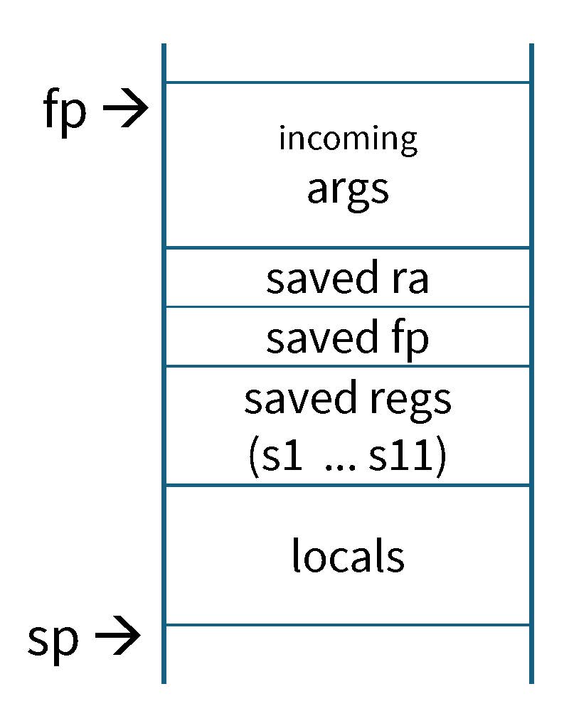
RISC-V Registers
- Return address:
x1(ra) - Stack pointer:
x2(sp) - Frame pointer:
x8(fp/s0) - First eight arguments:
x10-x17(a0-a7) - Return result:
x10-x11(a0-a1) - Callee-save free regs:
x18-x27(s2-s11) - Caller-save free regs:
x5-x7,x28-x31(t0-t6) - Global pointer:
x3(gp) - Thread pointer:
x4(tp)
Caches
The Memory Bottleneck
Remember our overview of computer architecture styles, where we assumed that each step in an instruction execution could happen in about one clock cycle? The assumption then was that it took about the same length of time to: fetch an instruction; decode it into control signals and access the register file; actually perform an arithmetic/logic operation like adding or multiplying two numbers; load or store to memory, if necessary; and write results back to the registers.
We can now tell you that this was a convenient fiction. While many of these stages do take about a cycle, there are important exceptions. For example, while it is easy to implement an integer addition circuit within one clock period (even at today’s multi-gigahertz clock frequencies), multiplication and division can often take several cycles. Think something like 3 to 15 cycles, depending on the complexity of the operation and the clock frequency.
But most importantly, accessing a computer’s memory is way slower than everything else. Loading or storing a single value to/from main memory takes hundreds of cycles on a modern computer. Because practical programs access memory every few instructions, this means that the performance of the memory system is an enormous factor in the performance of a computer system.
There are two big reasons why main memory is so slow: it is far away from the processor (both physically and metaphorically), and it uses a different physical technology. The result is that on-chip memory is fast, small, and expensive; off-chip (main) memory is slow, large, and cheap. For more on this fundamental trade-off, see our previous notes on the memory hierarchy.
SRAM vs. DRAM
One of the features of the memory hierarchy’s trade-off is a difference in manufacturing technology. Data storage on the CPU uses a technology called static RAM (SRAM), which is just built out of transistors—the same stuff that we make logic gates and registers out of. The ubiquitous technology for off-chip memory is dynamic RAM (DRAM). DRAM is a completely different technology that works by manufacturing arrays of tiny capacitors and periodically filling them with charge.
We already mentioned that SRAM is small, fast, and expensive while DRAM is large, slow, and cheap. But it’s worth dwelling for a moment on the sheer magnitude of the differences between the two.
- Speed: Accessing a value in SRAM typically takes roughly on the order of 0.5 nanoseconds. And in general, accessing any element in an SRAM is equally fast. In DRAM, accessing the first value in a DRAM array can take tens of nanoseconds. Subsequently accessing nearby values can be faster.
- Size: A typical size for an on-chip SRAM is roughly on the order of 1 MB. Even an entry-level laptop in 24 comes with 16 GB of DRAM.
- Cost: A rough estimate for the cost of DRAM storage is $3 per GB. It’s hard to pin down a good estimate for the cost of SRAM alone, because it usually comes with logic, but a good ballpark estimate is in the order of thousands of dollars per GB.
Because the trade-off is so extreme, it makes sense that computers would want to have some of each. An all-DRAM computer would be way too slow, and an all-SRAM computer would be way too expensive. Carefully combining memories of different speeds can have a huge impact on the cost/performance trade-off of a system.
Locality
This lecture is about caching, a technique that adds an intermediate-sized memory between registers and main memory. The idea is to build, out of SRAM, a place to put data that we access frequently. Then we’ll automatically transfer data from main memory (DRAM) to the cache (SRAM) so that most accesses, on average, can find their data in the cache.
To make this work, we will need a policy for automatically predicting which data is likely to be accessed frequently in the future. The key principle that caches will exploit is locality. Locality is a common pattern in real software that says that similar data is likely to be accessed close together in time.
Computer architects distinguish between two different forms of locality. Both of them are assumptions about how “normal” programs are likely to behave:
- Temporal locality: If a program accesses a given value, it is likely to need to access the same value again sometime soon.
- Spatial locality: If a program accesses a given value, it is likely to access nearby values in memory (i.e., addresses that are numerically close to the original address) sometime soon.
To illustrate the difference, consider this program:
int total = 0;
for (int i = 1; i < n; i++) {
  total += a[i];
}
return total;
Let’s think about the accesses to total and a[i].
Do these accesses exhibit spatial or temporal locality?
- The accesses to
totalhas high temporal locality because we access the same variable (the same address in memory) on every iteration of the loop—i.e., separated by only a few instructions. - The
a[i]accesses have high spatial locality because we are repeatedly, and close by in time, accessing nearby addresses in memory. When the program loadsa[i], it will very soon ask loada[i+1], whose address is only 4 bytes away.
Locality is an extremely general principle. Maybe you can think a little bit about other situations in your life that seem to exhibit temporal or spatial locality. Common examples of mechanisms for exploiting locality in everyday life include refrigerators, backpacks, and laundry hampers.
Hits & Misses
The idea with a cache is to try to “intercept” most of a program’s memory accesses. A cache wants to fulfill as many loads and stores as it can directly, using its limited pool of fast SRAM. In rare conditions where it does not have the data already, it reluctantly forwards the request on to the larger, slower main memory.
In the presence of a cache, every memory access that a program executes is either a cache hit or a cache miss:
- A hit happens when the data already exists in the cache, so we can fulfill the request quickly.
- A miss is the other case: the data is not already in the cache, so we have to send the request on to DRAM.
A cache’s purpose in life is to maximize the hit rate (or, equivalently, minimize the miss rate).
A Hierarchy of Caches
A single cache is good, so multiple caches must be better! Remember, there is a fundamental trade-off between memory size and speed. So modern computers don’t just have one cache at a single point in this trade-off space; they use several different caches of different sizes (and therefore different speeds). These are layered into a hierarchy.
It is common for modern machines to have three levels of caching, called the L1, L2, and L3 caches. The L1 cache is closest to the processor, smallest, and fastest. It is not unheard of to tack on an L4 cache. There are diminishing returns eventually, so this doesn’t go on forever.
In the L1 cache, it is also common for computers to separate the data and the instructions into separate caches. The data and instructions coexist in main memory, so it is totally reasonable to have a single L1 cache for both. But it turns out that the locality patterns for accessing instructions and data are so different that, to maximize performance, computer architects have found it helpful to keep them separate. You will sometimes see these separate caches abbreviated as the L1I and L1D cache.
Direct-Mapped Cache
We have talked a lot about the goals of a cache; let’s finally talk about how caches work. We’ll start with a simple style of cache called a direct-mapped cache. In this kind of cache, every address in main memory is mapped to exactly one location in the cache.
Let’s say we have 64-bit memory addresses, and we have a cache that can store \(2^n \ll 2^{64}\) values. To state the obvious, it is impossible for every memory address to get its own entry in the cache! So we need some policy to map memory locations onto cache locations. In a direct mapped cache, this is a many-to-one mapping.
Here’s the policy: we will split up the memory address, and we will use the least significant \(n\) bits of the address to determine the cache index, i.e., the location within the cache where this data will go. We have \(2^n\) cache locations, and there are \(2^n\) possible values of these \(n\) bits, so each value gets its own entry in the cache. We will then call the other \(64-n\) bits the tag; we will need these to disambiguate which address a given cache entry is currently holding.
We’ll implement the hardware for our cache so that each of the entries has 3 values: the tag, a valid bit, and the actual data. Let’s visualize a tiny 4-entry (\(n=2\)) cache like this:
| index | valid? | tag | data |
|---|---|---|---|
| 11 | |||
| 10 | |||
| 01 | |||
| 00 |
Here’s what these columns mean:
- The index is literally just the index of the cache entry. (This never changes.)
- The valid bit indicates whether that cache entry currently holds meaningful data at all. 0 means invalid (“don’t pay attention to this at all; nothing to see here”) and 1 means valid (“I am currently holding some cached data”). The invalid state is useful at program startup, when the cache doesn’t hold anything at all (all entries are invalid).
- The tag bit is those other \(64-n\) bits of the current value in the cache entry. That is, every cache entry could contain one one of \(2^{64-n}\) different memory addresses; the tag tells us which one it currently is.
- The data is the current value at that memory address. (This is the raison d’être of the cache!)
Now, to access a memory address \(a\), we’ll execute this algorithm:
- Split the address \(a\) into an index \(i\) (\(n\) bits) and a tag \(t\) (the other \(64-n\) bits).
- Look in entry \(i\) of the cache.
- Is the entry valid (is the valid bit 1)? If not, stop and go to main memory (this is a miss).
- Does the entry’s tag equal \(t\)? If not, stop and go to main memory (this is also a miss).
- The line is valid and the tag matches, so this is a hit. We can use the data from this cache entry and avoid going to main memory.
Filling the Cache
On a cache miss, we need to fetch the value from main memory. (Let’s only consider loads for now; we’ll handle stores later.) Because this is slow, we want to avoid doing this again in the future. So, we want to do something called filling the cache entry. After fetching the data from main memory, do these things:
- Look in entry \(i\) of the cache (again).
- Is the entry valid? If so, there is already some data here, and we will take its place. This is called an eviction. (We will discuss more about what to do about evictions in the next section.)
- Set the valid bit to 1 (regardless of what it was before), to indicate that it contains real data now.
- Set the tag to \(t\), to disambiguate which data it holds.
- Set the data to the value we got from main memory.
This way, subsequent accesses to the same address will hit. This is the way that caches exploit temporal locality, i.e., nearby-in-time accesses to the same address.
Example
To keep this example tractable, let’s pretend we only have 4-bit addresses (not 64). We’ll stick with a 4-entry cache, so the least-significant 2 bits are the index.
What happens when you execute this sequence of loads? Assume you start with en empty cache, where every entry is invalid. Label each access as a hit or a miss. Also, note each time an eviction occurs.
- load 1100
- load 1101
- load 0100
- load 1100
It can be helpful to draw out the four-column table above and update it after every access.
Larger Blocks
Our little cache is already pretty good at exploiting temporal locality, but we haven’t yet done anything about spatial locality. In our example above, when we access address 1100 and then immediately access 1101, both are misses even though the memory locations are “neighbors.” Under the hypothesis that many accesses in real applications will have spatial locality, we can extend the cache design to hit more often.
Here’s the idea. So far, every entry in our cache has only held a single memory address (and therefore only a single byte of data). Let’s generalize it to hold an entire block (a.k.a. line) of data, i.e., \(2^b\) bytes.
Before, we split the address into two pieces: the tag and the \(n\)-bit index. We will now split it into three. Listing from most-significant position to least-significant: the tag, the \(n\)-bit index, and the \(b\)-bit offset within the block.
You can visualize all of memory being broken up into \(2^b\)-byte blocks. The block is the unit of data that we will transfer to and from the cache. For example, when we fill data from main memory into the cache, we will fetch the entire \(2^b\)-byte block that contains \(a\) and put it into the cache. Now, loading a single byte brings in a bunch of neighbors—on the assumption that it’s likely that the program will soon need to access those neighbors.
The algorithm for accessing the cache remains the same; we just have to change the way we chunk up the address. And when we return data from the cache, we will use the least-significant \(b\) bytes as an offset to decide which byte from the block to return.
Example
Let’s return to our 4-byte cache from above. Let’s keep the design using 4 entries, but let’s make every entry store a 2-byte block instead of a single byte. That means our little 4-bit addresses now consist of 1 tag bit, 2 index bits, and 1 offset bit.
If you visualize this cache as a table, it looks exactly the same:
| index | valid? | tag | data |
|---|---|---|---|
| 11 | |||
| 10 | |||
| 01 | |||
| 00 |
The big difference now is that the “data” column stores 2-byte blocks. (The tag column now only stores 1 bit.)
Try simulating the same sequences of accesses again. Label the hits and misses:
- load 1100
- load 1101
- load 0100
- load 1100
Keeping Comparisons Fair
In this example, we cheated a bit: by doubling the size of the blocks, we double the total size of the cache. This means the cache is twice as big and twice as expensive. To make a fair comparison, between two cache designs, you’ll want to keep the total number of bytes the same. So if you double the block size, you should halve the number of entries.
Handling Stores
So far, we have only talked about loads (reads from memory). What about stores?
Writing to a cache works mostly the same as reading, except that we have a few choices to make.
- When we store to a block that is not already in the cache (a store miss), should we fill it (bring the block into the cache) or just send the write to memory? If so, this is called a write-allocate policy. Write-allocate caches make the (very reasonable) hypothesis that programs that write a given memory location are likely to read it again in the near future. If not, this is called a no write-allocate policy.
- When we store, should we just update the data in the cache, or should we also immediately send it to memory? The “immediately send all stores to main memory” policy is called write-through and it’s pretty simple. The other policy, where we just update the cache, is called write-back and it’s slightly more complicated.
The rest of this section will be about write-back caches. The write-back policy is a good idea in general because it means that you can avoid a lot of costly stores to main memory. It’s extremely popular for this reason. But it requires extra bookkeeping to deal with the fact that main memory and the cache can get “out of sync.”
Here’s the idea for keeping the cache and main memory in sync. We will add yet another value to our cache entries (another column in our table): the dirty bit. A cache entry is clean when it is in sync with main memory and dirty when it might disagree with main memory. Here’s how you can visualize the write-back cache:
| index | valid? | dirty? | tag | data |
|---|---|---|---|---|
| 11 | ||||
| 10 | ||||
| 01 | ||||
| 00 |
We will need to add these details to our algorithm for accessing the cache:
- When you fill a cache entry, initially set its dirty bit to 0. (The entry currently agrees with main memory.)
- Whenever you store to an entry in the cache, set its dirty bit to 1. (We are avoiding writing to main memory, so now a disagreement is possible.)
- Whenever you evict an entry from the cache, check its dirty bit. If the entry is clean, do nothing. If it’s dirty, write the data back to main memory then.
Example
Let’s try out a write-back policy with this sequence of accesses. Use our cache setup with 2-byte blocks as above.
- load 1100
- store 1101
- load 0100
- load 1100
Fully Associative Cache
All the caches we’ve seen so far have been direct-mapped: every block in main memory has exactly one cache entry where it might live. You may have noticed that these caches have a lot of evictions. Even when there is theoretically plenty of space in the cache, the fact that every block has only one option for where to live means that conflicts on these entries seem to happen all the time.
The opposite style of cache is a fully associative cache, where any memory address could use any entry in the cache. The index is no longer relevant at all; every cache entry could hold any address. When we divide up the address, you no longer take \(n\) bits for the index; the entire \(64-b\) bits are one gigantic tag.
We will also change the cache-access algorithm. Where the direct-mapped algorithm says “look at entry \(i\),” the fully associative version must look at every single entry in the cache, because the block we’re interested in might be anywhere.
Example
Let’s return to our 4-entry cache (with 2-byte blocks). In a fully associative version, because the indices are irrelevant, we can visualize it this way:
| valid? | tag | data |
|---|---|---|
There are 4 entries, all created equal, and they all might hold any address in all of memory. Let’s try the same sequence of loads again. Labels the hits and misses:
- load 1100
- load 1101
- load 0100
- load 1100
Replacement Policies
When you fill a block in a direct-mapped cache, there is only one choice of which existing block you should evict: the one that is in the (unique) entry where the block must live. In a fully associative cache, when the cache is full, you are now faced with a choice: which of the entries in the entire cache should we evict? An engineer designing a cache must decide on a replacement policy to answer this question.
There is an entire world of science dedicated to inventing cool eviction policies. The goal is to guess which block is least likely to be used again in the near future. And critically, it must make this decision efficiently—you can’t spend a lot of time thinking about which block to evict.
Some popular options include:
- Least-recently used (LRU): Keep track of the last time to access every block, and evict the one that was last used longest ago. The hypothesis is that, the longer a program goes not accessing a given block, the less likely it is to access it again soon. Unfortunately, LRU has a lot of overhead because you have to keep track of some kind of timestamp on every single block.
- Not most-recently used (NMRU): Like LRU, but only keep track of the most recently accessed block. When it comes time to evict, randomly pick some block that is not the most recent one you accessed. This makes somewhat worse decisions than LRU, but it’s a lot cheaper to implement and is popular for this reason.
- First-in first-out (FIFO): Keep track of which entry is oldest, and evict that one when needed.
The Costs of Associativity
Associativity is great! It leads to far fewer evictions. The problem is that it’s costly to implement in hardware. Because any block could go in any entry, we have to check all entries on every access to the cache. The hardware structure for implementing this “search all entries” operation is called a content-addressable memory (CAM). Because of the “search everywhere” nature of this operation, CAMs are expensive: large, hot, and slow. The cost scales with the number of entries, so it is only really practical to build fully associative caches when they are very small.
Set-Associative Cache
The final cache design we’ll consider strikes a balance between the direct-mapped and fully-associative extremes. A given address may live in exactly one entry in a direct-mapped cache; it may go in any entry in a fully associative cache; in a set-associative cache, it may live in one of a small number of entries grouped together into a set.
Let the number of entries in a set be \(k\). In caching terminology, our cache has \(k\) ways. If there are \(2^n\) total entries in our cache, then there are \(\frac{2^n}{k}\) sets. You can think of direct-mapped caches and fully associative caches as special cases:
- Direct-mapped: \(k = 1\), so there is only 1 way. There are \(2^n\) sets with a single block each.
- Fully associative: \(k = 2^n\), the it’s a \(2^n\)-way cache with only 1 (giant) set.
The usual way to visualize a set-associative cache is with a 2D grid of entries: one row per set, one column per way. Returning to our 4-entry cache with 2-byte blocks, we can make a visualization by copying and pasting two two-entry tables side by side:
| way 0 | way 1 | |||||
| index | valid? | tag | data | valid? | tag | data |
| 1 | ||||||
|---|---|---|---|---|---|---|
| 0 | ||||||
There are still 4 entries in this cache; they are now just grouped into sets of 2. This also means that the number of index bits goes from \(n\) to \(n-\log_2(k)\) (in this case, from 2 to 1) and the tags get correspondingly larger.
Let’s again update the algorithm for accessing the cache. After calculating the index, we now have to look at the entire set at that index. That means searching through all the ways (columns in our grid) associated with the index. And when we fill the cache after a miss, we need to choose which way within the set to evict using a replacement policy, just like in a fully associative cache.
Example
Once again, let’s simulate the same series of accesses on our machine with 4-bit addresses. This time, we will use a 4-entry, 2-way set associative cache, with a block size of 2. Use an LRU replacement policy. Here’s the sequence of loads again:
- load 1100
- load 1101
- load 0100
- load 1100
Three Categories of Misses
To understand the performance of some code (or of a cache design), you often want to pay attention to the cache misses. They can often be the slowest part of the program. It can also be useful to break down the misses by why they missed.
The 3 classic categories conveniently all start with the letter C:
- Cold or compulsory misses happen because this is the first access to the given cache line.
- Conflict misses happen because the associativity is too low, and too many lines competed for the same set and evicted a line that the program needed later on.
- Capacity misses happen because the entire cache is too small for the working set, and no amount of associativity could have helped.
Here’s an algorithm you can use to decide which category a miss belongs to:
- Was this cache line ever loaded before?
- If no: it’s a cold miss.
- If yes: Would this access have missed in a fully associative cache?
- If no: it’s a conflict miss.
- If yes: it’s a capacity miss.
Understanding Cache Performance
With so many choices about how to design a cache, it can be useful to understand how well your cache is performing on average. You can characterize the overall performance by computing the average memory access time (AMAT) for the entire memory system. The average access time is:
\[ t_{\text{avg}} = t_{\text{hit}} + r_{\text{miss}} \times t_{\text{miss}} \]
Where:
- \(t_{\text{hit}}\) (hit time): the time it takes to access the cache. Cache hits take exactly this amount of time; cache misses take this time to check the cache and then more time to go to main memory.
- \(r_{\text{miss}}\) (miss rate): the fraction of accesses that are misses.
- \(t_{\text{miss}}\) (miss penalty): the time it takes to retrieve data from a lower memory structure (i.e., a lower level cache, main memory).
For example, if it take 1 ns to access the cache and 50 ns to access main memory, and 95% of accesses hit, then the average access time is \(1 + 0.05 \times 50 = 3.5\) ns.
You can also extend this reasoning to multi-level cache hierarchies. Say you have an L1 cache and an L2 cache. From the perspective of the L1 cache, \(t_{\text{miss}}\) is the time it takes to access the rest of the cache hierarchy, i.e., to try accessing at L2. So you can calculate the average access time at the L2 cache and then use this average time as \(t_{\text{miss}}\) in the L1 access time calculation.
Cache Design
Designing an effective caching system is incredibly complex. Architects need to balance the total size of the cache, the block size, the amount of associativity (i.e., number of ways), the replacement policy, the write policy, the number of levels of cache, and whether to have a unified cache or not. All of these attributes affect cache performance in different ways. The definition of AMAT tells us that in order to improve cache performance we either need to:
- decrease the hit time,
- decrease the miss rate,
- and/or decrease the miss penalty.
Let’s consider the impact of increasing the block size on cache performance in a direct-mapped cache. Assume that the total cache size is fixed. A larger block size means that the cache has few entries (lines), but each entry contains more data. This results in fewer tags, so less overhead, as well as fewer cold misses thanks to prefetching. So, a larger block size could reduce the miss rate if a large portion of the cache misses are cold misses.
However, because a larger block size results in fewer entries, the likelihood of a conflict miss increases. If the working set of the program’s memory doesn’t fit within the cache, then too large of a block size could end up increasing the miss rate instead of decreasing it! A larger block size also results in a larger miss penalty as it takes longer to fetch a larger block from main memory.
OS Processes
So far in 3410, we have been operating under the ridiculous notion that a computer only runs one program at a time. A given program gets to own the computer’s entire memory, there is only a single program counter (PC) keeping track of a single stream of instructions to execute.
You know from your everyday computing life that this is not how “real” computers work. They can simultaneously run multiple programs with their own instructions, heap, and stack. The operating system (OS) is, among other responsibilities, the thing that makes it possible to run multiple programs on the same hardware at the same time. The next part of the course will focus on this mechanism: how the OS and hardware work together to work on multiple things concurrently.
Executable vs. Process
When you compile the C code you have written this semester, an executable file is produced. This is a file that contains the instructions (i.e., machine code) and data for your program. An executable is inert: it’s not doing anything; it’s just sitting there on your disk. You can copy an executable, rename it, attach it to an email, print it out, put it on a USB drive and send it through the US mail—anything you can do with any other file.
When you run an executable, that creates a process. A process is a currently running instance of a program. You can run the same executable multiple times and get multiple, concurrently executing processes of the same program. The different processes will share the same instructions and constant data, but they will have different heaps and different stacks (so different values of all their variables, potentially). It’s not just a file—you can’t print out a process or burn it to a CD. A process is something that occurs on a specific computer at a specific time.
Part of an operating system’s job is to provide processes with the illusion that they own the entire computer. That means that a process gets to use all of the machine’s registers without worrying about other processes using them at the same time. The OS manages the CPU’s program counter so it appears, to each process, to proceed normally through a given program’s instructions—without jumping willy-nilly to other programs’ instructions. Through a mechanism called virtual memory, every process gets the illusion of owning the entire \(2^{64}\)-byte memory address space. (Virtual memory will be covered later during the semester.)
The Process Lifecycle
What happens when you type ./myprog in your shell to launch an executable?
(Assume you already compiled an executable, myprog.)
The OS first must create a new process with the instructions and data from myprog.
The OS keeps track of all the processes on the system (running or not) in a
process list.
Each process gets an entry in this list called a process control block (PCB).
The PCB includes metadata like the process id (pid),
information about the user who owns the process,
the current state of the process (running, waiting, ready, etc.),
and so on.
To create a new myprog process, the OS allocates a new PCB and adds it to its
process list.
Next, the OS sets up the memory for the process. Recall that programs expect to have access to regions of memory for their stack, heap, global data, and instructions. So at the very least, the OS needs to take the instructions from the executable and put them into the text segment in memory. This per-process view of memory is called an address space — we will cover more about how to set up the memory address space for a process when we talk about virtual memory. Once completed, the OS updates the process’s state as ready in the PCB.
Finally, it’s time to run the process. The OS transfers control of the processor to the program’s first instruction by setting the program counter to that instruction’s address. At this point the process is running.
It can be helpful to think about a process’s state (as tracked by its PCB) as a state machine.
Process states include initializing, ready, running, waiting, and finished.
While setting up the PCB and the process’s memory, the OS places a new process in the initializing state.
Eventually, when this is all set up, the process becomes ready.
Then, when the OS decides to finally start a process, it sets the PCB’s state to running.
The OS uses the waiting state for processes that are waiting for the OS to complete some task on its behalf (such as I/O).
Finally, after main eventually returns, the process enters the finished state.
Context Switching
Many processes may be active at the same time, i.e., they may all have PCBs that are all ready. However, only one process can actually be running at a time. To give the illusion that multiple programs are running on your computer at the same time, the OS chooses some process to run for a short span of time, and then it pauses that process to allow another process run for some time. While the length of these time windows varies by OS and according to how busy the computer is, you can think of them happening every 1–5 ms if it helps contextualize the idea. The OS aims to give a “fair” amount of time to each process. This process (pun intended) is called time-sharing.
The act of changing from running one process to running another is called a context switch. Here’s what the OS needs to do to perform a context switch:
- Save the current process state. That means recording the current CPU registers (including the program counter) somewhere in memory.
- Update the current process’s PCB (to exit the running state).
- Select another process. (Picking which one to run is an interesting problem, and it’s the responsibility of the OS scheduler.)
- Update that PCB to indicate that the process is now in the running state.
- Restore that process’s state: read the previously-saved register values back from memory.
- Resume execution by jumping to the new process’s current instruction.
Context switches are not cheap. Again as a very rough estimate, you can imagine them taking about a microsecond, or something like a thousand clock cycles. The OS tries to minimize the total number of context switches while still achieving a “fair” division of time between processes.
Kernel Space & User Space
The kernel is a special piece of software that forms the central part of the operating system. You can think of it as being sort of like a process, except that it is the first one to run when the computer boots and it has the special privilege of managing all the actual processes. The kernel has its own instructions, stack, and heap.
Systems hackers will often refer to a separation between kernel space and user space.
OS stuff happens in kernel space: maintaining the PCBs, choosing which processes to run, and so on.
All the stuff that the processes do (every single line of code in myprog above, for instance) happen in user space.
This is a cute way to refer to the separation of code and responsibilities between the two kinds of code.
However, there is also an important difference in privileges:
kernel-space code has unrestricted access to all of the computer’s memory and to I/O peripherals.
It can read and write the memory of any process.
User-space code, because of kernel-space machinations, gets that aforementioned illusion of running in a sandbox where it does not have to worry about other processes.
In user space, each process receives a limited number of privileges from the kernel and must ask the kernel nicely to perform things like I/O or to communicate with other processes.
Processor ISAs provide mechanisms to enforce this distinction in privileges. For example, RISC-V has a special set of privileged instructions and registers that only kernel-space code is allowed to use. The CPU starts in a state where these instructions are allowed; when the OS starts a user-space process, it instructs the CPU to take away access to these instructions. When control eventually transfers back into kernel space, the CPU re-enables access to these privileged instructions.
System Calls, Signals, & Interrupts
On the previous episode, we began our journey to understand how the OS and hardware work together to work on multiple tasks concurrently. Recall that a process is a currently running instance of a program. Today, we will discuss how processes communicate with the OS.
System Calls
On their own, the only things that processes can do are run computational instructions and access memory. They do not have a direct way to manage other processes, print text to the screen, read input from the keyboard, or access files on the file system. These are privileged operations that can only happen in kernel space. This privilege restriction is important because it puts the kernel in charge of deciding when these actions should be allowed. For example, the OS can enforce access control on files so an untrusted user can’t read every other user’s passwords.
Processes can ask the OS to perform privileged actions on their behalf using system calls. We’ll cover the ISA-level mechanisms for how system calls work soon. For now, however, you can think of a system call as a special C function that calls into kernel space instead of user space. (Calling a “normal” function always invokes code within the process, i.e., either code you wrote yourself or code you imported from a library.)
Each OS defines a set of system calls that it offers to user space. This set of system calls constitutes the abstraction layer between the kernel and user code. (For this reason, OSes typically try to keep this set reasonably small: a simpler OS abstraction is more feasible to implement and to keep secure.)
In this class, we’re using a standardized OS abstraction called POSIX. Many operating systems, including Linux and macOS, implement the POSIX set of system calls. (We’ll colloquially refer to it as “Unix,” but POSIX is the actual name of the standard.)
For a list of all the things your POSIX OS can do for you, see the contents of the unistd.h header.
That’s a collection of C functions that wrap the actual underlying system calls.
For example, consider the write function.
write is a low-level primitive for writing strings to files.
You have probably never called write directly, but you have used printf and fputc, both of which eventually must use the write system call to produce their final output.
Process Management
There are system calls that let processes create and manage other processes. These the big ones we’ll cover here:
exitterminates the current process.forkclones the current process. So after youfork, there are two nearly identical processes (e.g., with nearly identical heaps and stacks) running that can then diverge and start doing two different things.execreplaces the current process with a new executable. So after youexeca new program, you “morph” into an instance of that program.execdoes not create or destroy processes—the kernel’s list of PCBs does not grow or shrink. Instead, the current process transforms in place to run a different program.waitpidjust waits until some other process terminates.
fork
The trickiest in the bunch is probably fork.
When a process calls fork(), it creates a new child process that looks almost identical to the current one:
it has the same register values,
the same program counter (i.e., the same currently-executing line of code),
and the same memory contents (heap and stack).
A reasonable question you might ask is:
do the two processes (parent and child) therefore inevitably continue doing exactly the same thing as each other?
What good is fork() if it can only create redundant copies of processes?
Fortunately, fork() provides a way for the new processes to detect which universe they are living in:
i.e., to check whether they are the parent or the child.
Check out the manual page for fork.
The return value is a pid_t, i.e., a process ID (an integer).
According to the manual:
On success, the PID of the child process is returned in the parent, and 0 is returned in the child.
This is why I kept saying the two copies are almost identical—the difference is here.
The child gets 0 returned from the fork() call,
and the parent gets a nonzero pid instead.
This means that all reasonable uses of fork() look essentially like this:
#include <stdio.h>
#include <unistd.h>

int main() {
    pid_t pid = fork();
    if (pid == 0) {  // Child.
        printf("Hello from the child process!\n");
    } else if (pid > 0) {  // Parent.
        printf("Hello from the parent process!\n");
    } else {
        perror("fork");
    }
    return 0;
}
In other words, after your program calls fork(), it should immediately check which universe it is living in:
are we now in the child process or the parent process?
Otherwise, the processes have the same variable values, memory contents, and everything else—so they’ll behave exactly the same way, aside from this check.
Another way of putting this strange property of fork() is this:
most functions return once.
fork returns twice!
exec
The exec function call “morphs” the current process, which is currently executing program A, so that it instead starts executing program B.
You can think of it swapping out the contents of memory to contain the instructions and data from executable file B and then jumping to the first instruction in B’s main.
There are many variations on the exec function; check out the manual page to see them all.
Let’s look at a fairly simple one, execl.
Here’s the function signature, copied from the manual:
int execl(const char *path, const char *arg, ...);
You need to provide the executable you want to run (a path on the filesystem) and a list of command-line arguments (which will be passed as argv in the target program’s main).
Let’s run a program! Try something like this:
#include <stdio.h>
#include <unistd.h>

int main() {
    if (execl("/bin/ls", "ls", "-l", NULL) == -1) {
        perror("error in exec call");
    }
    return 0;
}
That transforms the current process into an execution of ls -l.
There’s one tricky thing in the argument list:
by convention, the first argument is always the name of the executable.
(This is also true when you look at argv[0] in your own main function.)
So the first argument to the execl call here is the path to the ls executable file, and the second argument to execl is the first argument to pass to the executable, which is the name ls.
We also terminate the variadic argument list with NULL.
fork + exec = spawn a new command
The fork and exec functions seem kind of weird by themselves.
Who wants an identical copy of a process, or to completely erase and overwrite the current execution with a new program?
In practice, fork and exec are almost always used together.
If you pair them up, you can do something much more useful:
spawn a new child process that runs a new command.
You first fork the parent process, and then you exec in the child (and only the child) to transform that process to execute a new program.
The recipe looks like this:
fork()- Check if you’re the child. If so,
execthe new program. - Otherwise, you’re the parent. Wait for the child to exit (see below).
Here that is in code:
#include <stdio.h>
#include <unistd.h>
#include <sys/wait.h>

int main() {
    pid_t pid = fork();
    if (pid == 0) { // Child.
        if (execl("/bin/ls", "ls", "-l", NULL) == -1) {
            perror("error in exec call");
        }
    } else if (pid > 0) { // Parent.
        printf("Hello from the parent!");
        waitpid(pid, NULL, 0);
    } else {
        perror("error in fork call");
    }
    return 0;
}
This code spawns a new execution of ls -l in a child process.
This is a useful pattern for programs that want to delegate some work to some other command.
(Don’t worry about the waitpid call; we’ll cover that next.)
waitpid
Finally, when you write code that creates new processes, you will also want to wait for them to finish.
The waitpid function does this.
You supply it with a pid of the process you want to wait for (and, optionally, an out-parameter for some status information about it and some options),
and the call blocks until the process somehow finishes.
It’s usually important to waitpid all the child processes you fork.
Try deleting the waitpid call from the example above, and then compile and run it.
What happens?
Can you explain what went wrong when you didn’t wait for the child process to finish?
Signals
Whereas system calls provide a way for processes to communicate with the kernel, signals are the mechanism for the kernel to communicate with processes.
The basic idea is that there are a small list of signal values, each with its own meaning: a thing that the kernel (or another process) wants to tell your process. Each process can register a function to run when it receives a given signal. Then, when the kernel sends a signal to that process, the process interrupts the normal flow of execution and runs the registered function. Some signals also instruct the kernel to take specific actions, such as terminating the program.
There are also system calls that let processes send signals to other processes. (In reality, that means that process A asks the kernel to send the signal to process B.) This way, signals act as an inter-process communication/coordination mechanism.
Here are the functions you need to send signals:
kill(pid, sig): Sendsigto processpid.raise(sig): Sendsigto myself.
To receive signals, you set up a signal handler function with the signal function.
The arguments are the signal you want to handle and a function pointer to the code that will handle the signal.
Here’s an example of a program that handles the SIGINT signal:
#include <stdio.h>
#include <stdlib.h>
#include <signal.h>
#include <unistd.h>

void handle_signal(int sig) {
    printf("Caught signal %d\n", sig);
    exit(1);
}

int main() {
    signal(SIGINT, handle_signal); // Set up the signal handler for SIGINT.
    while (1) {
        printf("Running. Press Ctrl+C to stop.\n");
        sleep(1);
    }
    return 0;
}
The important bit is this line:
signal(SIGINT, handle_signal);
This line asks the kernel to register a function we’ve written so that it will run in response to the SIGINT signal.
Interrupts
We just discussed signals: the mechanism that the kernel uses to communicate with user-space processes. Recall that, when your process receives a signal, it interrupts the normal flow of execution and runs the signal-handler function that you previously registered. How does this actually work? How does the kernel interfere with the execution of a process in between instructions, take control, and forcibly move the program counter to some other code?
Signals use a more general (and extremely important) mechanism called interrupts. As the name implies, they are the mechanism that the kernel uses to interrupt the execution of a running process, which is otherwise minding its own business and running one instruction after another, and make it do something else.
Here’s a conceptual way to think about how interrupts work. You can think of a CPU as executing a loop: fetch an instruction, execute that instruction, and then go back to the top of the loop. To deal with interrupts, CPU add an extra step to this conceptual loop: fetch an instruction, execute that instruction, check to see if there are any interrupts to handle, and then go back to the top of the loop. That is, you can imagine that there is some place where the CPU can look to see if there is an interrupt to deal with, and it checks for this indicator between the execution of adjacent instructions. When there is an interrupt to handle, the CPU transfers control to some code that can handle the interrupt.
What Are Interrupts For?
The OS and hardware uses interrupts to deal with exception conditions (what happens if your program runs out of memory? or executes an illegal instruction that the CPU cannot interpret?) and to support kernel-mediated services like I/O. Here are a few reasons why interrupts are helpful:
- They are more efficient than busy-waiting, i.e., just looping until something happens. If you’re waiting for a packet to arrive from the network, for example, you can execute other work until the packet arrives—at which point the OS can interrupt you to deliver the packet.
- They make it possible to handle events in the real world immediately. When the mouse moves, for example, the OS and hardware can interrupt the currently executing process to make sure the cursor appears to move on screen (instead of waiting patiently for the currently-running program to be done, which would make for a terribly janky mouse cursor).
- Interrupts are critical for multitasking, i.e., running multiple processes at once. Interrupts are what OS kernels use to perform periodic context switches between concurrent processes to fairly share CPU time between them.
As a result, systems use interrupts for a very wide variety of reasons, some of which are “exceptional” (e.g., when a program tries to execute an illegal instruction or references an unmapped virtual memory address) and others that are totally normal (e.g., to handle I/O or when it’s time to do a context switch).
Requesting Interrupts with System Calls
We also previously discussed system calls: the mechanism that user-space code uses to invoke kernel-space functionality. The underlying mechanism for system calls also uses interrupts. The ISA typically provides a special instruction that processes can use to request an interrupt. When the hardware executes this instruction, it immediately transitions to kernel mode to handle the system call.
To decide which system call to make and to pass arguments to it,
OSes define a syscall-specific calling convention.
This is different from the ordinary calling convention that governs the calling of ordinary functions.
If you’re curious, Linux’s manual page for the syscall C function lists its calling conventions for every architecture that Linux supports.
In RISC-V, the special instruction for making system calls is named ecall.
It has no operands.
The Linux syscall convention for RISC-V says:
a7contains the system call number. This decides which kernel functionality we want to invoke. For example, the syscall number forwriteis 64, and the number forexecveis 221.- Arguments to the system call go in
a0througha5. - The return value goes in
a0, just like in the “ordinary function” calling convention.
You can see a full list of available system calls on the syscalls(2) manual page.
Then, to find the corresponding syscall number, the authoritative source is the unistd.h header file in the Linux source code:
search for #define __NR_<call> <number>.
You can also try
this big, searchable syscall table that covers all the architectures Linux supports (use the “riscv64” column).
The corresponding manual page tells you the arguments for the syscall, expressed as a C function signature.
An Example
Let’s handcraft a system call in RISC-V assembly using ecall.
We will use the Linux write system call to output characters to the console.
If we look in unistd.h, it tells us that the syscall number for write is 64.
The manual page says that this system call takes 3 arguments:
ssize_t write(int fd, const void buf[.count], size_t count);
There is the file descriptor, a pointer to the characters to output, and the number of characters. The file descriptor 0 is the standard output stream, i.e., it’s how we print to the console. Let’s write a function that always outputs to file descriptor 1 (standard output) and always prints exactly 1 character. Here are the assembly instructions we need:
  addi a7, x0, 64  # syscall number: write
  addi a0, x0, 1   # first argument: fd
  mv   a1, t0      # second argument: buf
  addi a2, x0, 1   # third argument: count
  ecall
We set the syscall number register, a7, to 64.
Then we provide the three arguments: file descriptor 0, a pointer (here I’m assuming it comes from t0), and length 1.
Finally, we use ecall to actually invoke the syscall.
Here’s a complete assembly file that wraps these instruction in a function for printing one-character strings:
.global printone
printone:
  mv t0, a0        # save the function argument: a character pointer

  # Make a system call: write(1, t0, 1)
  addi a7, x0, 64  # syscall number: write
  addi a0, x0, 1   # first argument: fd
  mv   a1, t0      # second argument: buf
  addi a2, x0, 1   # third argument: count
  ecall

  ret
You can use this assembly from C code by writing a function declaration for it, like this:
int printone(char* c);

int main() {
    printone("h");
    printone("i");
    printone("\n");
    return 0;
}
You can compile and run the whole program by combining the C file and the assembly file:
rv gcc -o printone printone.c printone.s
This program prints something to the console without ever importing any headers or using the C standard library at all. Pretty cool!
Virtual Memory
We have previously said that part of the operating system’s job is give each process the illusion that it is running alone on the hardware. This concept is called virtualization: the OS runs on the physical hardware and provides an abstraction of virtual hardware for each process to run on. The OS virtualizes a single CPU by scheduling multiple concurrent processes to interleave their execution and orchestrating context switches between them.
This lecture is about how to virtualize the memory: i.e., how the OS creates the illusion, for every process, that the process has exclusive access to its own memory. The goal of a virtual memory system is that every process should have its own memory address space. In other words, we want the address 0xCAFED00D in process A to refer to different data from 0xCAFED00D in process B. (Maybe you can think about how bad life would be without virtual memory. Every process would need to carefully avoid using any addresses in use by any other process. And any process could freely access the memory of any other process. Shockingly, this is how many popular OSes worked until as late as the ’90s, and it was as terrible as it sounds.)
Virtual vs. Physical Memory Addresses
Here’s the overall strategy. We will make a distinction between the virtual address space for each process and the physical address space for the actual machine:
- Each process will operate in its own address space, meaning that it thinks in terms of its own \(2^{64}\) memory locations. We will call these addresses virtual addresses.
- The actual main memory has some number of bytes available—probably much fewer than \(2^{64}\). We will call the addresses of these “real” storage locations physical addresses.
The OS and hardware will collaborate to construct a mapping between virtual and addresses and physical addresses.
That is, for every process, we will create a table that describes, for every virtual address, the physical address where that data can be found.
The hardware has a special structure, called the memory management unit (MMU), that can translate from virtual to physical addresses.
Whenever a process tries to load or store an address V (e.g., it uses an ld or sb instruction with memory address V),
the hardware will automatically perform a virtual-to-physical memory address translation to find the corresponding physical address P.
It will then load or store the “real” memory location P.
This scheme means that programs never see physical addresses. They only know about virtual addresses, and all their instructions load and store those addresses. The hardware transparently translates all of these loads and stores into physical addresses to find the actual data. This way, processes can remain blissfully unaware of where their data is actually stored in the hardware and just think in terms of their own, private address space.
The data structure that describes the virtual-to-physical address translation is called the page table (for reasons we will see in a moment). The OS is responsible for setting up the page table and putting it into (physical) memory so the hardware knows where it is. When user-space code is running, the hardware then uses the page table to perform address translation. This is how the OS and hardware collaborate to implement virtual memory.
Pages and Page Tables
Let’s take a closer look at how page tables and address translation work.
An extremely inefficient way to set up a page table would be to explicitly record, for every virtual address in use, the corresponding physical address. This would mean that every single byte in a process’s virtual address space has its own, special mapping onto a specific byte in physical memory. This strawperson scheme is too fine grained: for one thing, it would require 8 bytes of address-mapping metadata for every byte of data!
Instead, VM systems divide all of memory up into chunks called pages. To give you a rough idea of the granularity, an extremely popular page size is 4 kB (4,096 bytes). You can imagine all of a process’s virtual address space, and all of the physical address space, divided up into these equally-sized chunks. Page tables work by mapping entire virtual pages (4 kB ranges of virtual addresses) onto physical pages (4 kB ranges of physical addresses).
As with cache blocks, this mapping works by dividing up the memory address. 4,096 is (2^{12}), so we will divide all memory addresses into the most-significant 52 bits and the least-significant 12 bits. The least-significant 12 bits are the offset within the page. The remaining (most-significant) 52 bits are the page number.
Some terminology: we will use virtual page number (VPN) and physical page number (PPN) when we’re talking about those non-offset bits in the address, depending on whether we’re referring to virtual or physical memory.
The page table then maps VPNs to PPNs. To translate a virtual address to a physical address, do these steps: split it into the page number (VPN) and the offset, translate the page number (from VPN to PPN), and then add the offset back on. Now you have a physical address.
The Memory Management Unit
The memory management unit (MMU) is the hardware structure that is responsible for translating virtual addresses to physical addresses. It uses a page table to perform this translation. But each process has its own page table—so how does the MMU know where to find the right page table at any given time?
The OS stores each process’s page table in main memory. (The kernel has the special privilege of using physical addresses directly, so it does not need to worry about address translation for its own accesses!) Then, when it performs a context switch, the OS needs to tell the hardware which page table is currently active for the process it is about to switch to. There is a special register that stores the (physical) address of the currently-active page table. The OS sets this register during each context switch to point to the relevant page table. Then, the MMU uses this register whenever it needs to perform address translations.
In RISC-V, this register is called satp (Supervisor Address Translation and Protection). Note that the RISC-V privileged ISA changed the name of sptbr (Supervisor Page Table Base Register) to satp (Supervisor Address Translation and
Protection) to reflect the fact it could be used for more than just paging.
You can read more about it in the privileged instruction manual.
Fancier Page Tables
You now know the basic mechanism for virtual memory: how the OS creates the illusion that every process is running in isolation. The rest of this lecture is about various extensions that build on the basic VM mechanism to do other cool stuff that systems need to do.
To support all of these extensions, VM systems enrich the page table with more metadata. Remember that the main thing that a page table needs to do is to map VPNs to PPNs: i.e., a basic version is nothing more than an array of PPNs indexed by VPN. In real systems, the page table also includes other stuff, like this:
- A valid bit, indicating whether the virtual page is mapped at all. (Kind of like the valid bit in a cache.) It is an error to access an address within an unmapped page.
- Protection bits. The OS can decide whether each page can be read, written, and/or executed. Think of this as 3 extra bits, named R, W, and X. It is an error, for example, to try to store to an address within a page whose W bit is 0. The X bit is especially important for security: the OS can prevent processes from executing instructions within writable memory (sometimes called the W^X restriction) to make it harder to exploit bugs that would otherwise trick the program into running malicious instructions.
You may also be worried that this sounds like a lot of data. If there are really \(2^{52}\) virtual pages, do we really need \(2^{52}\) entries in our page table? In practice, systems will compress this data structure using a multi-level page table, which lets the system omit chunks of entries for large ranges of invalid addresses. The details of these compressed data structures is out of scope for CS 3410.
Swap & Page Faults
There is one cool thing that virtual memory system enables that goes beyond isolating processes. VM can also let you transparently “overflow” your memory. If you run a bunch of programs that, all together, use more memory than you actually have available in your machine, the OS can transparently move some of their data to the disk. This mechanism is called swap, i.e., it works by swapping chunks of processes’ memory out to disk. (This mechanism is also called paging, because it involves moving pages around. Pages that are in memory are paged in or swapped in and pages that are relegated to the disk are paged out or swapped out.)
Processes do not need to be aware that their data has been swapped out. They can continue to pretend that they have unlimited access to all their memory. The OS takes care of moving data between main memory and the disk. Remember, accesses to the disk are much, much slower than main memory—so the OS tries to intelligently place frequently-accessed data in memory. The goal ends up very much like CPU caches: it exploits temporal and spatial locality to maximize the number of accesses that go to main memory, not to disk.
The strategy for implementing swapping is to mark paged-out memory as invalid in the page table. Remember that, when the CPU tries to access any virtual address, it must first consult the page table to perform protection checks (and to do the address translation). When the program accesses an invalid virtual page, a page fault occurs. The CPU uses an interrupt to transfer control to the kernel to handle the page fault.
There are many reasons that a page fault could occur.
It could be that the address is just unallocated:
the process never malloc’d that address.
(If you have ever gotten a segmentation fault error when running your C program (who hasn’t?), that’s what this means.)
The OS looks at its internal data structures to decide what happened:
i.e., to check whether the invalid virtual page is actually stored somewhere on disk.
If so, it pages in that data and then lets the process continue.
To page in new data, the OS reads the page from disk and places it into physical memory. This can mean evicting a different virtual page of data; the OS needs a replacement policy, just like in an associative cache, to decide which page to evict.
Because disks are so much slower than memory, swapping a page in takes a long time—think tens of milliseconds, roughly, or tens of thousands of clock cycles. So frequent swapping can seriously harm a program’s performance. And it’s enough time that the OS scheduler will likely try to find other work to do while the disk request is outstanding.
At a high level, swap lets disk join the memory hierarchy at a level below main memory. DRAM is sort of a cache for the hard disk; the CPU cache acts the same way for the DRAM; registers are kinda like a cache for the cache. It’s caches all the way down.
Sharing
Here is another cool thing that virtual memory enables. The page table translates virtual addresses to physical addresses; there is nothing intrinsic that requires this mapping to be injective. That is, if virtual address A in process X maps to physical address P, then it’s totally possible for virtual address B in process Y to map to exactly the same physical address P!
This observation implies a scheme where different processes can share the same data, without actually duplicating the data in main memory. Say that N different processes happen to need the same B bytes of data. With virtual memory, we can do this by spending only B total bytes of physical memory! Without VM, each process would need its own copy, for a total of N×B bytes.
There are a few situations where this kind of sharing is extremely useful in practice:
- Libraries. Multiple processes often need the same library code; they can share a read-only memory region to save space that would otherwise be duplicated for the library’s code.
- Inter-process communication. Process A can communicate with process B by writing into a memory region that the two processes share.
Multicore
One of the two motivations we used when introducing threads was the idea of harnessing parallel hardware to make computations go faster. Parallelism is important because the overwhelming majority of computers in the modern world are parallel. When was the last time (if ever) that you saw a laptop for sale with a single-core CPU? Core counts like 8 are much more common today. Even the Apple Watch has a dual-core processor and Samsung Watch has five cores! And on the other end of the spectrum, server processors have core counts like 96 and 192. The result is that, when performance matters, parallelism is the only way to take full advantage of the hardware.
Multicore processors are designed to enhance computing performance by incorporating multiple cores within a single chip. Each core can execute instructions independently, allowing for parallel processing of tasks. This architecture is crucial for modern computing devices, which require high performance for various applications.
Amdahl’s Law
However, Amdahl’s Law highlights the limitations of performance improvement in parallel computing. It states that the overall performance gain from parallelism is limited by the portion of the task that must be executed serially. This law serves as a caution against expecting unlimited scaling by adding more parallel resources. For example, if we had a matrix sum that had 80% of its computation which could be partitioned and performed in parallel, but there was also 20% that was scalar and needed to be peformed in serielly, then eventually the serial portion would dominate and limit performance. In this particular example, 5x speedup would be the maximum no matter much we divided the parallel portion.
Multicore and Parallelism
The need for multiple cores in devices like smartphones is driven by the demand for higher computing power. Moore’s Law, which predicts the exponential growth of transistors on a chip, has been a guiding principle in the development of multicore processors. Further, increasing clock frequencies was once the primary strategy for improving performance. However, increasing clock frequencies has hit its limits due to heat and power constraints. See the breakdown of Dennard Scaling.
Other methods to increase performance included instruction level parallelism such as pipelining, multi-issue (also known as superscalar) processors, out-of-order execution, speculative execution, register renaming, and many other techniques. Take CS 4420 (ECE 4750) to learn more. Utlimately, these techniques used too much power and dissipated too much heat. Instead, modern RISC based processors with simple pipleines and without a lot of these advanced ILP approaches have become dominant again for multicore processors because they better balance performance and power.
Threads and Synchronization
Parallel programming involves partitioning work so that all cores have tasks to execute. Coordination and synchronization are crucial to manage communication overhead and ensure efficient execution. Writing parallel programs requires careful consideration of the underlying architecture to optimize performance.
Threads are a fundamental mechanism for exploiting parallelism. They allow multiple sequences of instructions to be executed concurrently. Synchronizing parallel programs involves using atomic instructions and hardware support to manage access to shared resources, preventing race conditions and ensuring correct execution.
Writing parallel programs requires understanding threads and processes, critical sections, race conditions, and mutual exlusion (mutexes). These concepts help in managing the execution of multiple threads and ensuring that they do not interfere with each other.
Cache Coherency
One of the challenges in multicore systems is cache coherency. When multiple processors cache shared data, they might see different values for the same memory location, leading to inconsistencies. Ensuring cache coherency is essential for maintaining the integrity of data across all cores.
Cache Coherency
In modern computing systems, parallelism and synchronization are crucial concepts, especially in multicore architectures. Multicore systems feature multiple processor cores, each equipped with its own cache such as a level-one (L1) cache. This setup allows for increased computational power and efficiency. However, it also introduces the challenge of cache coherency.
Cache coherency refers to the problem that arises when multiple processors cache shared data. Each processor may see different values for the same memory location, leading to incoherent views of memory. This issue is particularly relevant in shared memory multiprocessors (SMP), where multiple cores share a single physical address space. In typical SMP configurations, there are 1-4 processor dies, each containing 2-8 cores. The hardware provides a single physical address space for all processors, which necessitates mechanisms for data sharing, coordination, and scalability.
Cache Coherency Protocols
Cache coherency is a complex but essential aspect of multicore systems. It requires that reads to a particular memory location return the most recently written value, which is a difficult problem to solve. Various protocols, such as snooping and directory-based protocols, have been developed to address this issue. Each protocol has its advantages and limitations, and the choice of protocol depends on the specific requirements of the system. Snooping protocols, in particular, are where each cache monitors bus reads and writes. When a cache detects a bus read or write, it responds accordingly to maintain coherence. We discuss two protocols, Valid-Invalid (VI) and Modified-Shared-Invalid (MSI). In both the VI and MSI cache coherence prototocols, we are assuming write-back caches.
Valid-Invalid (VI) Cache Coherence Protocol
The VI (valid-invalid) protocol is a simple coherence protocol with two states: valid (V) and invalid (I). When a processor loads or stores a block, it transitions the cache block to the valid state. If another processor wants to read or write the block, the original processor must give up its copy, writing to memory if the block is dirty, and transitioning the cache block to the invalid state.
Modified-Shared-Invalid (MSI) Cache Coherence Protocol
The MSI (modified-shared-invalid) protocol improves upon the VI protocol by introducing a third state: modified (M). This state allows a processor to have a local dirty copy of a block. The shared (S) state allows multiple read-only copies of a block, while the invalid (I) state indicates that the block is not present in the cache.
Both the VI and MSI protocols maintain cache coherency for a single memory address, where a read returns the latest write for that particular address. However, cache coherency is not sufficient for to maintain atomicity over multiple instructions. See the notes on synchronization.
False Sharing
False sharing occurs when two or more processors share parts of the same cache block but not the same bytes within that block. This can lead to inefficient “ping-pong” behavior, where processors repeatedly invalidate each other’s cache lines. Careful data placement can mitigate false sharing, though it is challenging to achieve.
Threads
The next several lectures will all be about doing multiple computations at once. As we saw in the previous lecture, real software needs to deal with concurrency (managing different events that might all happen at the same time) and parallelism (harnessing multiple processors to get work done faster than a single processor on its own). Compared to sequential code, concurrency and parallelism require fundamental changes to the way software works and how it interacts with hardware.
Here are some examples of software that needs concurrency or parallelism:
- A web server needs to handle concurrent requests from clients. It cannot control when requests arrive, so they may be concurrent.
- A web browser might want to issue concurrent requests to servers. This time, the software can control when requests happen—but for performance, it is a good idea to let requests overlap. For example, you can start a request to server A, start a request for server B, and only then wait for either request to finish. That’s concurrency.
- A machine learning application wants to harness multiple CPU cores to make its linear-algebra operations go faster: for example, by dividing a matrix across several cores and working on each partition in parallel.
Threads are an OS concept that a single process can use to exploit concurrency and parallelism.
What Is a Thread?
A thread is an execution state within a process. One process has one or more threads. Each thread has its own thread-specific state: the program counter, the contents of all the CPU registers, and the stack. However, all the threads within a process share a virtual address space, and they share a single heap.
One way to define a thread is to think of it as “like a process, but within a process.” That is, you already know that processes have separate code (so they can run separate programs), register states, separate program counters, and separate memory address spaces. Threads are similar, except that threads exist within a process, and all threads within a process share their virtual memory. All threads within a process are running the same program (they have same text segment)—they may just execute different parts of that program concurrently. Threads also share the data segment and file descriptors.
When a process has multiple threads, it has multiple stacks in memory. Recall the typical memory layout for a process. When there are multiple threads, everything remains the same (the heap, text, and data segments are all unchanged) except that there are multiple stacks coexisting side-by-side in the virtual address space.
The threads within a process share a single heap. That means that threads can easily communicate through the heap: one thread can allocate some memory and put some data there and then simply let another thread read that data. This shared memory mechanism is both incredibly convenient and ridiculously error prone. (We will get more experience with the problems it can cause later.)
The thread’s state includes the registers (including the program counter and the stack pointer). The OS scheduler takes care of switching not only between processes but also between the threads in a process. When the computer has multiple CPU cores (as all modern machines do), the OS may also choose to schedule concurrent threads onto separate cores when there are multiple threads with work to do.
Why Threads?
You may be wondering why we might use threads. Further, do threads make sense with just a single core (spoiler: yes!)?
The key benefit of threads over processes is that all threads within a process run the same program and share virtual memory.
This encourages a natural program structure, as opposed to using processes, for example.
It would be rather clunky and tedious to fork() off separate child processes to update the screen, fetch data, and receive user input.
Processes need to use an inter-process communication mechanism (e.g., signals, pipes, files) to pass data between each other.
These mechanisms also tend to be significantly more expensive performance-wise.
Since they share memory, threads make it easy to write programs which must logically concurrent tasks. Even on a system with a single core, threads can make programs more responsive and efficient. One thread could be processing data in a buffer while another is fetching new data to push to the end of the same buffer. Yet another thread could be responsible for updating the screen.
pthreads
Now that we know what threads are and why they are important, how do we program with them?
Unsurprisingly, Unix provides a standard library, called POSIX Threads, or affectionately, pthreads, that contains procedures for managing threads and synchronizing them.
Next week we will dive deeper into the world of parallel programming, but for now, we will stick with the basics.
You can read the entire pthread.h header to see what’s available.
Spawning & Joining Threads
The pthread_create function launches a new thread.
It’s a tiny bit like fork and exec for processes, but for threads within the current process instead of creating new subprocesses.
Here’s its signature:
int pthread_create(pthread_t* thread, pthread_attr_t* attr,
    void *(*thread_func)(void*), void* arg);
We’ll revisit the other arguments next week, but the important ones for now are:
- The first argument,
thread, is apthread_tpointer to initialize. This struct is what the parent will use to interact with its brand-new child thread. - The third argument,
thread_func, is a function pointer to the code to run in the new thread. The thread function has to have a specific signature:void* thread_func(void* arg). Thevoid*argument and return types are C’s way of letting the thread function receive and return “anything.”
It’s OK (for now) to pass NULL for the other parameters.
So the basic recipe for spawning a new thread looks like this:
void* thread_func(void* arg) {
    // code to run in a new thread!
}

// ...

pthread_t thread;
pthread_create(&thread, NULL, thread_func, NULL);
Whenever you spawn a thread, you will also want to wait for it to finish, a.k.a. join the thread.
There is a pthreads call for that too, in the pthread_join function:
int pthread_join(pthread_t thread, void** out_value);
We will again ignore the second parameter for a moment (it can be NULL).
The first parameter is the pthread_t value that we previously initialized with pthread_create.
The call to pthread_join blocks until the given thread finishes.
Putting it all together, here’s a complete program that launches a thread and then properly waits for it to finish:
#include <stdio.h>
#include <pthread.h>

void* my_thread(void* arg) {
    printf("Hello from a child thread!\n");
    return NULL;
}

int main() {
    printf("Hello from the main thread!\n");

    pthread_t thread;
    pthread_create(&thread, NULL, my_thread, NULL);
    pthread_join(thread, NULL);

    printf("Main thread is done!\n");
    return 0;
}
In order to compile this program, we need to include the -lpthread option to tell GCC to link the pthreads library:
rv gcc threads.c -o threads -lpthread
When we run the program, three messages are printed in order:
Hello from the main thread!
Hello from a child thread!
Main thread is done!
Synchronization
When you program with threads, you are using a shared-memory parallelism programming model. This means that multiple streams of instructions are running simultaneously, and they can both read and write the same region of memory. As we discussed last time, this programming model is relatively natural; threads don’t need to do anything special to communicate with each other and they all run the same program (usually different parts of the same program). Do not be deceived by this apparent simplicity though, as programming with threads is notoriously complex and error prone.
While each thread executes the program sequentially, there is (almost) no ordering or timing guarantees between threads. This problem leads to a whole class of bugs which are hard to reason about and may be impossible to reproduce. In this lecture, we will focus on recognizing and fixing these problems with synchronization.
Atomicity
Consider the following C program which spawns two threads that both concurrently increment the variable x:
*x += 1;
If the value x points to starts out at 0 before these two threads run, it would be nice if we could be guaranteed that that *x contained 2 after both threads finish.
But, as you know, *x += 1 is not a single action that your machine takes all at once.
You need to break it down into at least three steps:
load the value, add 1 to it, and then store it back to memory.
What can happen as these three steps from the two threads interleave?
For example, consider what happens if this ordering events happens:
- thread 1 loads the value
xpoints to - thread 2 loads the same value
- thread 1 increments the value
- thread 2 increments it
- thread 1 stores the modified value back to address
x - thread 2 stores its modified value back to address
x
What would the value of *x be then?
If this is not the intended behavior—if the programmer intended both copies of *x += 1 to take places as a single unit, resulting in the final value 2—then this is a violation of atomicity.
That is, the programmer might intend for an action like *x += 1 to be atomic: to happen all at once, without the ability for any thread to observe or interfere with the intermediate states between the beginning and the end of the operation.
But in C (and in the equivalent assembly), this is not an atomic operation: it consists of several smaller observations, and other threads can interfere in the middle.
Mutual Exclusion
Synchronization is a technique to avoid the problems that arise from shared-memory parallelism, such as atomicity violations. There are many forms of synchronization, and this lecture will explore a few of them.
An extremely popular form of synchronization is mutual exclusion, or mutex for short, also known as locking. The idea is that we want to delimit parts of the code where only one thread can be running at a time. Imagine that C had a special construct for mutual exclusion; then we might write this:
mutex {
  x += 1;
}
This would mean that only one thread would be allowed to be running inside those curly braces at a time. The region of code protected by mutual exclusion (the code inside the braces inside this imaginary construct) is called a critical section. So if thread 1 entered the critical section, and then thread 2 arrived at the top of the section, it would need to wait until thread 1 left the critical section before it could enter.
Can you convince yourself that this mutual exclusion would fix the atomicity problems from our example? If we enforce mutually exclusive execution of that critical section, is that enough? (It is.)
Sadly, C does not have a built-in mutex construct.
Instead, we need to use a library or build it ourselves.
A Failed Attempt
Here’s a naive way that you might try to implement mutual exclusion: use a lock variable to keep track of whether someone is currently occupying the critical section.
Something like this:
int lock = 0;

while (lock) {}  // Wait for the lock to be free.
lock = 1;        // Acquire the lock.
*x += 1;         // Critical section here.
lock = 0;        // Release the lock.
That should do it, right? What happens if two different threads run this code concurrently?
It doesn’t work.
Imagine that both threads first encounter the while statement, and they both bypass it before setting lock to 1.
So we have failed to enforce mutual exclusion.
It’s possible to fall down a deep rabbit hole of techniques for implementing mutual exclusion. A famous example is Peterson’s algorithm, which works by combining one flag variable per thread (instead of one shared flag variable).
However, these custom algorithms for mutual exclusion are neither necessary nor sufficient. They are not necessary because CPUs provide special instructions just for implementing synchronization mechanisms such as mutual exclusion. They are not sufficient because CPUs implement optimizations that typically mean that any synchronization mechanism implemented using ordinary loads and stores, instead of the special instructions, cannot work reliably.
This insufficiency is a deep topic of its own that is mostly out of scope for CS 3410, we briefly discused cache coherency. but here’s a brief summary. Please skip this paragraph unless you are super duper curious about an entirely separate branch of computer science. In a multiprocessor system, it takes a while for each processor to publish its memory stores so that they can be read by other processors. (The architectural component to blame is a store buffer.) That means that each CPU can read its own writes immediately, but other processors see these updates only after a delay. This results in a memory consistency model that allows updates to appear “out of order” to remote processors. Processors have therefore developed special instructions that bypass these optimizations and, at the cost of performance, force certain memory accesses to happen in a sequentially consistent order. All correct synchronization implementations, therefore, must use these special instructions instead of ordinary load and store instructions.
The key takeaway here is that in order to implement correct synchronization primitives, we need hardware support.
Atomic Instructions
RISC-V provides two basic atomic instructions to support the implementation of synchronization operations such as mutual exclusion.
They are called lr, for load reserved, and sc, for store conditional.
These two instructions work together to provide the basic mechanisms required to implement any style of synchronization.
(In other ISAs, this pattern is called load-link/store-conditional.)
The instructions come in different accesses sizes; for example, lr.w and sc.w are the word-sized (32-bit) versions.
Here’s what the instructions do:
lr.w rd, (rs1): Load the 32-bit value at the address inrs1and put the value inrd. (So far, like a normallw.) Also, create a “reservation” of this address. (What is a “reservation”? Keep reading.)sc.w rd, rs2, (rs1): Store the value ofrs2at the address inrs1. (Again, so far, like a normal store.) But, also check whether a reservation of this address exists. If so, then the store proceeds as normal, and setrdto 0. (Call this a “success.”) If not, then cancel the store altogether: do not write anything at all the memory, and setrdto 1. (This is a “failure.”)
This “reservation” business is a mechanism for checking whether anyone else wrote to a given address.
While a reservation exists, think of the CPU carefully monitoring the given address to see if anyone else writes to that address.
If nobody writes to the address between the lr and the sc, the reservation is preserved and sc succeeds.
If somebody else does write to the given address, then the reservation is lost and sc fails.
lr.d / sc.d are equivalant to lr.w / sc.w except 64-bit instead of 32-bit.
Implementing Synchronization Operations
The usual way to use lr and sc together is to put them at the beginning and the end of some region of code, and then wrap the whole thing in a loop.
The loop lets you try the code repeatedly, until the sc succeeds.
If you’re careful, this can mean that the code surrounded by the lr/sc pair eventually executes atomically.
The pattern looks something vaguely like this:
loop:
  lr.w t0, (a0)
  # ... do something with t0 to compute t1 ...
  sc.w t2, t1, (a0)
  bnez t2, loop     # if the lr/sc failed, then try again
The memory address in this example is in register a0.
This little loop tries to do something with the value at this address and then store it back.
If any other thread ever interferes, then it gives up and tries again—over and over, until the operation succeeds.
The end result is that we get to perform an atomic operation on the value stored at the address in a0.
You will use this pattern to implement interesting synchronization operations, including mutual exclusion, in this week’s assignment. If you’re curious about other types of synchronization operations not covered in CS 3410, take CS 4410!
Parallel Programming
One of the two motivations we had when introducing threads was the idea of harnessing parallel hardware to make computations go faster. Parallelism is important because the overwhelming majority of modern computers are parallel. When was the last time (if ever) you saw a laptop for sale with a single-core CPU? Core counts like eight are much more common today. Even the Apple Watch has a dual-core processor. And on the other end of the spectrum, server processors have core counts like 96 and 192. As a result, when performance matters, parallelism is the only way fully utilize the hardware.
Now that you know about the “building blocks” for parallelism (namely, atomic instructions), this lecture is about writing software that uses them to get work done. In CS 3410, we focus on the shared memory multiprocessing approach, a.k.a. threads. There are many other programming models for writing parallel software out there, but the shared-memory approach is ubiquitous: because they represent an incremental extension of a sequential programming paradigm, they are kind of the “default” way for modern software to incorporate parallelism.
pthreads
Last week’s assignment was on implementing synchronization operations to support parallel programming. It turns out that Unix has a standard library, called POSIX Threads or, affectionately, pthreads, that implements many of these sync ops for you. This lecture is about moving up the abstraction hierarchy: now that you know how these building blocks work, we can grant ourselves permission to use the “standard” version.
You can read the entire pthread.h header header to see what’s available.
Let’s walk through the basics step by step.
Spawn & Join Threads
The pthread_create function launches a new thread.
It’s a tiny bit like fork and exec for processes, but for threads within the current process instead of creating new subprocesses.
Here’s the signature:
int pthread_create(pthread_t* thread, pthread_attr_t* attr,
    void *(*thread_func)(void*), void* arg);
We’ll come back to the other arguments, but the important ones for now are:
- The first argument,
thread, is apthread_tpointer to initialize. This struct is what the parent will use to interact with its brand-new child thread. - The third argument,
thread_func, is a function pointer to the code to run in the new thread. The thread function has to have a specific signature:void* thread_func(void* arg). Thevoid*argument and return types are C’s way of letting the thread function receive and return “anything.”
It’s OK (for now) to pass NULL for the other parameters.
So the basic recipe for spawning a new thread looks like this:
void* thread_func(void* arg) {
    // code to run in a new thread!
}

// ...

pthread_t thread;
pthread_create(&thread, NULL, thread_func, NULL);
Whenever you spawn a thread, you will also want to wait for it to finish, a.k.a. join the thread.
There is a pthreads call for that too, in the pthread_join function:
int pthread_join(pthread_t thread, void** out_value);
We will again ignore the second parameter for a moment (it can be NULL).
The first parameter is the pthread_t value that we previously initialized with pthread_create.
The call blocks until the given thread finishes.
Putting it all together, here’s a complete program that launches a thread and then properly waits for it to finish:
#include <stdio.h>
#include <pthread.h>

void* my_thread(void* arg) {
    printf("Hello from a child thread!\n");
    return NULL;
}

int main() {
    printf("Hello from the main thread!\n");

    pthread_t thread;
    pthread_create(&thread, NULL, my_thread, NULL);
    pthread_join(thread, NULL);

    printf("Main thread is done!\n");
    return 0;
}
There are no race conditions here; this program is properly synchronized and is guaranteed to print the three messages in order:
Hello from the main thread!
Hello from a child thread!
Main thread is done!
Arguments & Return Values
Thread functions take a void* argument and return a void* return value so that the parent can communicate with it.
You pass a pointer to the argument value to pthread_create, and pthreads will pass this along to the thread function’s argument.
Then, if you return a value from the thread function, the parent can receive that value through an “out-parameter” in pthread_join:
that is, the parent has to wait for the child to finish for the return value to become available.
Here’s an example of a thread that performs the incredibly heavy-duty work of multiplying an integer by 2:
#include <stdio.h>
#include <pthread.h>

void* doubler_thread(void* arg) {
    int* num = (int*)arg;
    *num = *num * 2;
    return arg;
}

int main() {
    int my_number = 21;
    printf("Before, my_number = %d\n", my_number);

    pthread_t thread;
    pthread_create(&thread, NULL, doubler_thread, &my_number);
    int* result;
    pthread_join(thread, (void**)&result);
    printf("Result returned: %d\n", *result);

    printf("After, my_number = %d\n", my_number);
    return 0;
}
The parent passes a pointer to my_number to the doubler_thread thread function.
The thread function then passes the same pointer right back to the parent.
While thread arguments are really important, to be honest, I don’t usually find thread return values all that useful. It’s usually easier to just use the thread argument: to pass a pointer to where the thread should write its results. You’ll see that happen in the rest of the examples in this lecture.
Launching Lots of Threads
You usually want to create many threads at once, not just one.
You still need one pthread_t per thread, so a good tactic is to use an array (on the stack or the heap) of these.
Use a loop to launch the threads with pthread_create,
and then another loop to wait for each one with pthread_join.
Here’s an example that launches one thread per number in a range to check if it’s prime (in the slowest way possible):
#include <stdio.h>
#include <pthread.h>
#include <stdbool.h>

#define NUMBERS 20

bool is_prime(int n) {
    for (int i = 2; i < n; ++i) {
        if (n % i == 0) {
            return false;
        }
    }
    return true;
}

typedef struct {
    int number;
    bool* prime_flags;
} my_thread_args_t;

void* prime_thread(void* args_in) {
    my_thread_args_t* args = (my_thread_args_t*)args_in;
    args->prime_flags[args->number] = is_prime(args->number);
    return NULL;
}

int main() {
    // We'll set `prime[i]` to true iff `i` is prime.
    bool prime[NUMBERS];

    // Launch a thread to check every number.
    pthread_t threads[NUMBERS];
    my_thread_args_t thread_args[NUMBERS];
    for (int i = 1; i < NUMBERS; ++i) {
        thread_args[i] = (my_thread_args_t){
            .number = i,
            .prime_flags = prime,
        };
        pthread_create(&threads[i], NULL, prime_thread, &thread_args[i]);
    }

    // Join all threads and print results when ready.
    for (int i = 1; i < NUMBERS; ++i) {
        pthread_join(threads[i], NULL);
        printf("%d is %s\n", i, prime[i] ? "prime" : "composite");
    }

    return 0;
}
This example also demonstrates another useful technique: defining your own little struct just to use as the argument to the thread function.
If thread functions could take multiple arguments, we might just do that.
But using a struct for the arguments is the next best thing.
Here, my_thread_args_t contains the number that the thread is supposed to process and a pointer to the results array where it should write.
To ensure that the argument struct remains “alive” for the entire duration of the thread, we also need an array to store all these my_thread_args_t values.
(It would not work, for example, to use a local variable inside the loop.)
Make Threads Do Coarse-Grained Chunks of Work
Threads are not free. Launching a thread takes time to coordinate with the OS; joining similarly costs waiting time; each running thread costs bookkeeping memory; and frequent context switching between threads adds overhead. And if you are aiming to fully harness a parallel CPU, it doesn’t help to have more threads than you have available hardware parallelism anyway.
It is therefore not a good idea to launch threads that only do a tiny amount of work, such as checking a single number for primality. Checking thousands or millions of numbers is perfectly practical, but launching millions of threads to check each one is not. In practical programming, you will want to divide a problem into coarser-grained chunks of work. Then you can launch a small number of threads—probably somewhere close to the number of cores in your machine.
For our primality example, it could make sense to divide up the numbers we need to check.
We can extend our my_thread_args_t struct to contain not just one number but a start/end interval.
Then, we just need to change our thread to loop over the range.
Here’s a full implementation:
#include <stdio.h>
#include <pthread.h>
#include <stdbool.h>

#define THREADS 8
#define NUMBERS 1024

bool is_prime(int n) {
    for (int i = 2; i < n; ++i) {
        if (n % i == 0) {
            return false;
        }
    }
    return true;
}

typedef struct {
    int start_number;
    int end_number;
    bool* prime_flags;
} my_thread_args_t;

void* prime_thread(void* args_in) {
    my_thread_args_t* args = (my_thread_args_t*)args_in;

    for (int n = args->start_number; n < args->end_number; ++n) {
        args->prime_flags[n] = is_prime(n);
    }

    return NULL;
}

int main() {
    // We'll set `prime[i]` to true iff `i` is prime.
    bool prime[NUMBERS];

    // Launch a thread to check chunks of numbers.
    pthread_t threads[THREADS];
    my_thread_args_t thread_args[THREADS];
    int numbers_per_thread = NUMBERS / THREADS;  // Hopefully they divide.
    for (int i = 0; i < THREADS; ++i) {
        thread_args[i] = (my_thread_args_t){
            .start_number = i == 0 ? 1 : i * numbers_per_thread,
            .end_number = (i + 1) * numbers_per_thread,
            .prime_flags = prime,
        };
        pthread_create(&threads[i], NULL, prime_thread, &thread_args[i]);
    }

    // Join all threads and print results when ready.
    for (int i = 0; i < THREADS; ++i) {
        pthread_join(threads[i], NULL);
        for (int n = thread_args[i].start_number;
             n < thread_args[i].end_number;
             ++n) {
            printf("%d is %s\n", n, prime[n] ? "prime" : "composite");
        }
    }

    return 0;
}
The nice thing about this version is that the problem size (the number of integers to check for primality) is not related to the thread count. So we can freely change the two parameters independently.
Concurrency Bugs
Sadly, parallel programming comes with an entirely new category of bugs to worry about. You have already seen atomicity violations, for example, and many other forms of concurrency bugs also lurk in shared-memory programming. In essence, the whole game of parallel programming is avoiding concurrency bugs without sacrificing too much of the awesome performance potential of parallel hardware.
A Racy Program
Let’s try changing our multithreaded primality checker to, instead of reporting which numbers are prime, just count how many primes exist in a range of numbers. Here’s the complete program:
#include <stdio.h>
#include <pthread.h>
#include <stdbool.h>

#define THREADS 8
#define NUMBERS 1024

bool is_prime(int n) {
    for (int i = 2; i < n; ++i) {
        if (n % i == 0) {
            return false;
        }
    }
    return true;
}

typedef struct {
    int start_number;
    int end_number;
    int* prime_count;
} my_thread_args_t;

void* prime_thread(void* args_in) {
    my_thread_args_t* args = (my_thread_args_t*)args_in;

    for (int n = args->start_number; n < args->end_number; ++n) {
        if (is_prime(n)) {
            (*(args->prime_count))++;
        }
    }

    return NULL;
}

int main() {
    int primes = 0;

    // Launch a thread to check chunks of numbers.
    pthread_t threads[THREADS];
    my_thread_args_t thread_args[THREADS];
    int numbers_per_thread = NUMBERS / THREADS;  // Hopefully they divide.
    for (int i = 0; i < THREADS; ++i) {
        thread_args[i] = (my_thread_args_t){
            .start_number = i == 0 ? 1 : i * numbers_per_thread,
            .end_number = (i + 1) * numbers_per_thread,
            .prime_count = &primes,
        };
        pthread_create(&threads[i], NULL, prime_thread, &thread_args[i]);
    }

    // Join all threads.
    for (int i = 0; i < THREADS; ++i) {
        pthread_join(threads[i], NULL);
    }

    // Print final prime count.
    printf("%d numbers in the range 1-%d are prime\n",
           primes, (NUMBERS - 1));

    return 0;
}
When I compiled and ran this program on my machine, it gave disturbingly inconsistent answers. Here are a few runs:
$ gcc -O2 threads-racy.c -o racy
$ ./racy
153 numbers in the range 1-1023 are prime
$ ./racy
163 numbers in the range 1-1023 are prime
$ ./racy
154 numbers in the range 1-1023 are prime
$ ./racy
167 numbers in the range 1-1023 are prime
$ ./racy
153 numbers in the range 1-1023 are prime
$ ./racy
159 numbers in the range 1-1023 are prime
$ ./racy
161 numbers in the range 1-1023 are prime
It’s bad enough that these answers are incorrect, but even worse, the program is nondeterministically incorrect.
The problem is reminiscent of the basic atomicity violation that we saw recently, but it actually indicates an even deeper problem.
Data Races
The fundamental problem in the buggy program above it can unsynchronized memory access. The formal name is a data race. Here’s a definition: a data race occurs when two different threads perform unsynchronized accesses to the same memory location, and at least one of those accesses is a write.
To understand this definition, is an be useful to think through things that are not data races:
- Memory accesses within a single thread. Memory accesses can of course be buggy for other reasons, but they are not data races!
- When different threads access different memory locations. In our original primality check program, for example, different threads wrote to different
primes[i]indices. But no two threads ever tried to write to the same index, so there was no data race. - Multithreaded reads of the same data. It is always OK for different threads to share read-only data. The only situations that are data races are when one thread writes and the other thread reads and when both threads write.
The final criterion is that unsynchronized qualifier. This has a more nuanced definition, but it broadly means that there are no synchronization operations (such as locks) protecting the data. The implication is that you can always fix data races by adding synchronization.
The line in our program with the data race is this one:
(*(args->prime_count))++;
Let’s check the four parts of our definition:
- Multiple threads run this line.
- The access is unsynchronized: we haven’t done anything to ensure ordered access.
- The accesses go to the same memory location. (There is only one
prime_countvariable.) - Although the
++syntax makes it slightly harder to see, this line both reads and writes the variable.
So this is indeed a data race.
Data races are undefined behavior in C (and C++). That means that they are equally problematic as a violation of the heap laws: use-after-free bugs, out-of-bounds accesses, and so on. The compiler is allowed to assume your program does not have races and transform and bases its optimizations on that assumption.
The consequence is that you cannot reason about the behavior of racy programs; they can do anything. To write working parallel software, you must avoid data races.
Locks in pthreads
You can fix data races by adding synchronization. We could even use the spin-lock mutex that is on your current assignment. But pthreads also provides a mutual exclusion lock. There are three steps to use a pthreads lock:
- Initialize it. You can use the
pthread_mutex_initfunction or thePTHREAD_MUTEX_INITIALIZERconstant. - Acquire the lock with the
pthread_mutex_lockfunction. - When your critical section is done, release the lock with the
pthread_mutex_unlockfunction.
To fix our racy program above, we can declare a new mutex in main:
pthread_mutex_t mutex = PTHREAD_MUTEX_INITIALIZER;
Then, we’ll need to pass this mutex along to each thread by adding it to our my_thread_args_t struct.
Within each thread, we’ll acquire and release the mutex to protect a critical section:
pthread_mutex_lock(args->mutex);
(*(args->prime_count))++;
pthread_mutex_unlock(args->mutex);
We now have a properly synchronized program with no data races. If we run this program, it reliably gets the right answer:
$ gcc -O2 threads-mutex.c -o mutex
$ ./mutex
173 numbers in the range 1-1023 are prime
$ ./mutex
173 numbers in the range 1-1023 are prime
$ ./mutex
173 numbers in the range 1-1023 are prime
Catching Races with Thread Sanitizer
The section below talks about ThreadSanitizer. While it works fine on most architectures, it currently does not work on RISC-V.
To catch other forms of undefined behavior such as out-of-bounds accesses, we recommend enabling sanitizers in the compiler. Is there a similar way to detect data races?
Fortunately, yes:
ThreadSanitizer is a feature built into some compilers that does exactly this.
Unfortunately, it also doesn’t (yet) work in the CS 3410 RISC-V container.
But if you like and you have a recent compiler set up on your host machine, you can enable ThreadSanitizer with -fsanitize=thread.
For example, this will find the data race in our buggy example above (before we added the lock):
$ clang -g -fsanitize=thread threads-racy.c -o racy
$ ./racy
==================
WARNING: ThreadSanitizer: data race (pid=56484)
  Write of size 4 at 0x00016dd9efe0 by thread T2:
    #0 prime_thread threads-racy.c:28 (racy:arm64+0x100003c04)

  Previous write of size 4 at 0x00016dd9efe0 by thread T1:
    #0 prime_thread threads-racy.c:28 (racy:arm64+0x100003c04)
[...]
This error indicates that line 28 of threads-racy.c had a data race with itself.
Producer/Consumer Parallelism
Locks and critical sections are only one way to coordinate work between multiple threads. This section will build up toward a different style.
One limitation in our approach so far to dividing work into chunks is imbalance between threads. Our primality program, for example, takes as long as the slowest thread. Larger numbers take longer to check, so the earlier chunks will run faster than the later chunks. Dealing with this kind of imbalance is a major challenge in parallel programming.
One parallel programming technique to help automatically deal with imbalance is the producer/consumer pattern. The idea is that you will have one thread producing the work to do and \(n\) parallel threads consuming the work items and actually doing the work. You need a data structure to keep track of the work and to intermediate between the producer and the consumers.
We’ll start by designing that data structure and then build up to a new automatically-balancing implementation of our primality checker.
Circular Buffer
We need a queue data structure to intermediate between the producer and the consumers. The idea is that the producer will push work items on to the tail of the queue, and consumers will pop items from the head.
A sensible way to implement a bounded-size queue is with a circular buffer (a.k.a. a ring buffer). The idea is to allocate an array of \(n\) elements, and to hope that you never need to have more than \(n\) things in your queue at once. Then, you keep track of two indices: the head and the tail of the queue. They “wrap around” the \(n\)-element array.
Here’s a sample implementation of a bounded buffer without any parallelism involved.
We’ll need a struct to keep track of the state:
typedef struct {
    int* data;
    int capacity;  // The size of the `data` array.
    int head;      // The next index to pop.
    int tail;      // The next index to push.
} bounded_buffer_t;
Here are the functions to push into and pop from the queue:
void bb_push(bounded_buffer_t* bb, int value) {
    assert(!bb_full(bb));
    bb->data[bb->tail] = value;
    bb->tail = (bb->tail + 1) % bb->capacity;
}

int bb_pop(bounded_buffer_t* bb) {
    assert(!bb_empty(bb));
    int value = bb->data[bb->head];
    bb->head = (bb->head + 1) % bb->capacity;
    return value;
}
The functions work by advancing the head or tail index by one and then “wrapping around” the capacity-sized array.
There is a critical detail here represented by the assert calls.
(You can imagine simple implementations of bb_full and bb_empty: the buffer is empty if the head and tail indices are equal, for example.)
We really don’t want to push into a full buffer or pop from an empty queue.
When we take this data structure into a parallel context, we will want to handle these conditions by waiting for some other thread to do push or pop before proceeding with our own operation.
A Simple Lock and Busy Waiting
One way to make the producer/consumer pattern work is to wrap all our accesses to the queue in a lock, just like any other shared data structure.
We’ll start by extending the queue data structure:
typedef struct {
    int* data;
    int capacity;  // The size of the `data` array.
    int head;      // The next index to pop.
    int tail;      // The next index to push.

    pthread_mutex_t* mutex;
    bool done;
} bounded_buffer_t;
We add a mutex to protect the lock, and also a done flag to signal to consumers that there are no more items coming.
Next, we will implement variants of the bb_push and bb_pop functions that are safe to call from separate threads, and which block (wait) until they can succeed.
Our goal is to write a couple of thread functions like this:
void* producer_thread(void* arg) {
    bounded_buffer_t* buf = (bounded_buffer_t*)arg;
    for (int i = 0; i < NUMBERS; ++i) {
        printf("producing %d\n", i);
        bb_block_push(buf, i);
    }
    bb_finish(buf);
    return NULL;
}

void* consumer_thread(void* arg) {
    bounded_buffer_t* buf = (bounded_buffer_t*)arg;
    while (1) {
        bool done;
        int number = bb_block_pop(buf, &done);
        if (done)
            break;
        printf("consuming %d\n", number);
    }
    return NULL;
}
The producer thread pushes the numbers 0 through NUMBERS-1 into the queue.
Whenever the queue is full, bb_block_push should wait until there is room and then proceed.
The consumer thread pops one number at a time.
The bb_block_pop call blocks until there is at least one item in the queue to consume or until the done flag becomes true, in which case the thread should shut down.
Let’s look at bb_block_push first:
void bb_block_push(bounded_buffer_t* bb, int value) {
    pthread_mutex_lock(bb->mutex);

    // Spin to wait until the queue has room to push.
    while (bb_full(bb)) {
        // Release the lock for a moment to let other threads proceed.
        pthread_mutex_unlock(bb->mutex);
        pthread_mutex_lock(bb->mutex);
    }

    // Actually do the push.
    bb_push(bb, value);

    pthread_mutex_unlock(bb->mutex);
}
This is a busy waiting loop: we repeatedly check for there to be room in the queue, and when there finally is, then we push. The tricky thing I’ve done here is to briefly unlock and relock the buffer’s mutex. If we didn’t do this, no other thread could acquire the lock to pop, so we could never make progress.
The critical sections here (regions between a pthread_mutex_lock and pthread_mutex_unlock) are a little harder to see because of this trick.
But they protect all the shared state:
all the accesses to the buffer’s internal data happen with the lock held.
The bb_block_pop function looks somewhat similar:
int bb_block_pop(bounded_buffer_t* bb, bool* done) {
    pthread_mutex_lock(bb->mutex);

    // Spin to wait until queue has a value (or until we are done).
    while (bb_empty(bb) && !bb->done) {
        pthread_mutex_unlock(bb->mutex);
        pthread_mutex_lock(bb->mutex);
    }

    // Either we're done or we can pop.
    int value;
    if (bb->done) {
        *done = true;
        value = 0;
    } else {
        value = bb_pop(bb);
    }

    pthread_mutex_unlock(bb->mutex);
    return value;
}
One main difference here is that we also need to check for the done flag.
Because it’s shared state, that access also needs to be protected by the buffer’s mutex.
This implementation totally works. It is a little sad that we had to resort to busy-waiting, though: it is inefficient to need to repeatedly acquire a lock to check a condition until it happens to change. This should be a clue that a mutex alone may not be the perfect tool for the job.
Condition Variables
This is a perfect use case for a different synchronization construct: a condition variable. You always pair a condition variable with a lock. Condition variables let you temporarily release the lock while you wait for other threads to change some condition you care about. In this case, the condition we need to wait for is the fullness or emptiness of the buffer.
The pthreads library provides a pthread_cond_t type for condition variables.
Aside from initialization/destruction, there are three important operations:
pthread_cond_wait(cond, mutex): Call this function while you already holdmutex. The function temporarily releasesmutex, waits for a signal from another thread on the condition variablecond, and then re-acquiresmutex.pthread_cond_signal(cond): Signal (i.e., wake up) one thread that is currently waiting oncond.pthread_cond_broadcast(cond): Signal all threads that are waiting oncond.
An important thing to realize about the condition variable API is that it doesn’t say anything about whether an actual logical condition about your program is true or false. That’s up to you. It just handles the mechanics of waiting for the abstract idea of condition changes.
The Correct Way™ to use condition variables is to wait on them in a loop that checks your actual, logical condition to become true. Something like this:
pthread_mutex_lock(mutex);
while (!check_your_condition()) {
    pthread_cond_wait(cond, mutex);
}
do_stuff();  // Now you know `check_your_condition()` returned true.
pthread_mutex_unlock(mutex);
The specification for pthread_cond_wait allows for spurious wakeups:
the call can sometimes return even when nobody signaled.
That’s why it’s a good idea to always put your wait call in a loop that checks whether the condition actually changes.
It also lets other threads “err on the side of signaling”:
it is OK to signal a condition even if there’s a chance the logical condition did not actually change.
Because you know all the waiting threads will double-check the condition in their loops, you can feel safe in signaling even when you don’t strictly need to.
Using Condition Variables in the Producer/Consumer Pattern
Let’s try replacing the busy waiting in our producer/consumer program with condition variables.
We will associate two pthread_cond_t condition variables with our buffer in its definition:
typedef struct {
int* data;
int capacity; // The size of the `data` array.
int head; // The next index to pop.
int tail; // The next index to push.
pthread_mutex_t* mutex;
bool done;
pthread_cond_t* full_cv;
pthread_cond_t* empty_cv;
} bounded_buffer_t;
The two condition variables reflect two abstract states:
whether the queue is full and whether it is empty.
We’ll signal the full_cv condition variable when the buffer goes from full to non-full.
Similarly, we’ll signal empty_cv when it goes from empty to non-empty.
Here’s what the push function looks like with condition variables:
void bb_block_push(bounded_buffer_t* bb, int value) {
pthread_mutex_lock(bb->mutex);
while (bb_full(bb)) {
pthread_cond_wait(bb->full_cv, bb->mutex);
}
bb_push(bb, value);
pthread_mutex_unlock(bb->mutex);
pthread_cond_signal(bb->empty_cv);
}
The loop looks pretty similar; we just get to replace that unlock/lock pair with a pthread_cond_wait.
The wait call appears in a loop that checks the actual logical condition.
After the critical section finishes, we know that the queue’s emptiness may have changed, so we signal the empty_cv condition.
We can change the pop function in a similar way:
int bb_block_pop(bounded_buffer_t* bb, bool* done) {
pthread_mutex_lock(bb->mutex);
while (bb_empty(bb) && !bb->done) {
pthread_cond_wait(bb->empty_cv, bb->mutex);
}
int value;
if (bb->done) {
*done = true;
value = 0;
} else {
value = bb_pop(bb);
}
pthread_mutex_unlock(bb->mutex);
pthread_cond_signal(bb->full_cv);
return value;
}
This time, we need to signal the full_cv condition because, after this pop is done, the queue may have just gone from full to non-full.
The code is shorter this way, and the pthreads library can help put these threads to sleep while they’re waiting. Awesome!
Deadlock
We have seen two types of concurrency bugs so far: atomicity violations and data races. This section is about a third kind. Deadlock is the name for the problem that happens when two different threads get stuck waiting for the other.
Here’s the general scenario. Imagine a situation with two threads, T1 and T2, that need to use some sort of shared resources, R1 and R2. The program wants to prevent concurrent use: i.e., only one thread can be using a resource at a given time. Now imagine that T1 is currently using only R1 and T2 is currently using only R2. Next, imagine that T1 also wants to start using R2, and that T2 wants to start using R1. Because R2 is busy, T1 must wait for T2 to be done with it. Similarly, because R1 is busy, T2 must wait. Neither thread can make progress, so neither can relinquish their reservation on either resource. So we are stuck.
An Example
We can turn this abstract idea into real code using locks. We’ll spawn two threads, and use two locks (representing the shared resources R1 and R2 above). The program looks like this:
#include <stdio.h>
#include <pthread.h>
pthread_mutex_t lock1 = PTHREAD_MUTEX_INITIALIZER;
pthread_mutex_t lock2 = PTHREAD_MUTEX_INITIALIZER;
void* thread1(void* arg) {
printf("Hello from a thread 1!\n");
pthread_mutex_lock(&lock1);
/*** Potential deadlock here! ***/
pthread_mutex_lock(&lock2);
pthread_mutex_unlock(&lock2);
pthread_mutex_unlock(&lock1);
return NULL;
}
void* thread2(void* arg) {
printf("Hello from a thread 2!\n");
pthread_mutex_lock(&lock2);
/*** Potential deadlock here! ***/
pthread_mutex_lock(&lock1);
pthread_mutex_unlock(&lock1);
pthread_mutex_unlock(&lock2);
return NULL;
}
int main() {
printf("Hello main!\n");
pthread_t threads[2];
pthread_create(&threads[0], NULL, thread1, NULL);
pthread_create(&threads[1], NULL, thread2, NULL);
pthread_join(threads[0], NULL);
pthread_join(threads[1], NULL);
printf("Main is done!\n");
return 0;
}
I’ve added a comment to mark the problematic point in both threads.
If both threads were to reach that point at the same time,
then thread1 would need to wait for thread2 to release lock2 and vice versa.
Deadlock!
If you try to compile and run this example, however, it will be hard to make this potential deadlock manifest. You have to get unlucky with the relative progress of the two threads. If one thread happens to finish before the other one even gets started, for example, there’s no deadlock here.
This is the worst kind of concurrency bug: the kind that manifests rarely. If the bug happens every time, that’s not great, but at least you can find it, reproduce it and fix it. If you have a bug manifest only once every N days or months, it’s hopeless: you can recreate exactly the same conditions that led to the bug and not be able to trigger the behavior so you can inspect it. As one recent example, here’s a blog post from some Netflix engineers about an intermittent concurrency bug (not a deadlock, but the point still stands). In that story, it was easier to just periodically kill the problematic processes than to find and fix the bug.
Just so we can prove it’s a problem, we can force the deadlock to happen every time by synchronizing the threads at the problematic point. Like this:
void* thread1(void* arg) {
printf("Hello from a thread 1!\n");
pthread_mutex_lock(&lock1);
barrier();
printf("Passed the barrier in thread 1!\n");
pthread_mutex_lock(&lock2);
pthread_mutex_unlock(&lock2);
pthread_mutex_unlock(&lock1);
return NULL;
}
void* thread2(void* arg) {
printf("Hello from a thread 2!\n");
pthread_mutex_lock(&lock2);
barrier();
printf("Passed the barrier in thread 2!\n");
pthread_mutex_lock(&lock1);
pthread_mutex_unlock(&lock1);
pthread_mutex_unlock(&lock2);
return NULL;
}
By using a barrier to make the threads reach the point just before they acquire the second lock, we can make the deadlock manifest deterministically.
A Rule for Avoiding Deadlock
The crucial mistake that makes our example above deadlock is that the threads acquire the locks in different orders.
thread1 has a lock1 critical section surrounding a lock2 critical section; thread2 acquires and releases the locks in the opposite order.
Think about what would happen instead if both threads acquired lock1 and then, within that critical section, had a smaller lock2 critical section.
It turns out that you can use this observation to concoct a rule for avoiding deadlocks when using mutexes:
- Decide on a total order among all your mutexes.
- Always acquire the mutexes in that order.
- Always release them in opposite order.
A different way of describing the third element in the rule is that, when critical sections overlap, one should always entirely contain the other—they should never partially overlap. So this is OK:
pthread_mutex_lock(&lock1);
// do stuff with one lock
pthread_mutex_lock(&lock2);
// do more stuff with both locks
pthread_mutex_unlock(&lock2);
// do even more stuff with just lock1
pthread_mutex_unlock(&lock1);
But this is not, because neither critical section entirely contains the other:
pthread_mutex_lock(&lock1);
// do stuff with one lock
pthread_mutex_lock(&lock2);
// do more stuff with both locks
pthread_mutex_unlock(&lock1);
// do even more stuff with just lock2
pthread_mutex_unlock(&lock2);
If you always “scope” your critical sections, and you always acquire your locks in a consistent order, you can avoid deadlock that arises from locks.
Input/Output (I/O)
Throughout this semester we have largely focused on the two main components of a Von Neumann architecture: the processor and memory. As we’ve said numerous times throughout the course of the semester, the processor does computations and memory stores data. This simplified presentation, while useful for pedagogical purposes, results in a computer that is frankly, pretty boring. We are lacking any way of providing inputs to our programs, so we are restricted to writing programs that produce the same result each time we run it. Similarly, our programs lack any way of returning any outputs. If we can’t interact with our programs, and they can’t interact with their environment, what is the point of running them at all?
I/O Devices
Real-life computers often have many I/O devices connected to it at any given time. You undoubtedly have a keyboard and mouse connected to your computer, for instance. These two I/O devices enable you, the user (a human), to provide direct input to the computer. You also likely have a microphone and webcam for audio and video inputs. Conversely, the computer might use your display/graphics, speakers, or even a printer to communicate with you, the user/human.
Modern computers also have a number of I/O devices that are used to communicate with other machines. For example, I would be surprised if your laptop didn’t come equipped with a network interface controller (NIC) to connect to the Internet with. You also (very) likely have at least one persistent storage device device, like a hard disk drive (HDD), solid-state drive (SSD), even a USB thumbdrive.
A common misconception is that memory and storage are interchangeable terms. While both refer to technologies that store data, they differ in their speed and volatility. Volatile memory requires power to maintain the stored information, whereas non-volatile (or persistent) storage will retain data without power. Memory generally refers to fast, volatile data storage technologies such as registers and DRAM. Storage, on the other hand, refers to slower, non-volatile (persistent) technologies like HDDs and SSDs.
I/O devices also vary wildly in how fast they can send and receive data. For example, keyboards only need to tell the computer which keys were pressed, so they only send about 100 bits/sec. Mice send about 3,800 bits/sec. Network devices work much faster with a data rate ranging from ~10 megabits/sec. all the way up to 400 gigabits/sec. HDDs are much slower in comparison with a data rate ranging from 800 megabits/sec. to 3 gigabits/sec.
The takeaway here is that while I/O devices come in all different shapes, sizes, and speeds, they enable a computer to interact with its environment and are thus essential for building interesting, useful computer systems.
Interconnects
Now that we’ve established that we need I/O devices, how do we actually integrate them into our computer system? We need some type of interconnect or bus to physically connect our processor and main memory together, in addition to a host of I/O devices. An interconnect consists of two main parts: a physical pathway that facilitates the actual data transfer, and a communication protocol to ensure that the data exchange is orderly. A common way of thinking of an interconnect is as a “data highway”. In this analogy, the physical pathway is the road itself and the communication protocol are all the traffic signs, lights, and pavement markings to prevent collisions and regulate the flow of traffic.
Attempt 1: Unified Memory and I/O Interconnect
As a first attempt, let’s do the simplest thing we can think of: connect the CPU, main memory, and all I/O devices on a single, unified memory and I/O interconnect. Consider the diagram below.
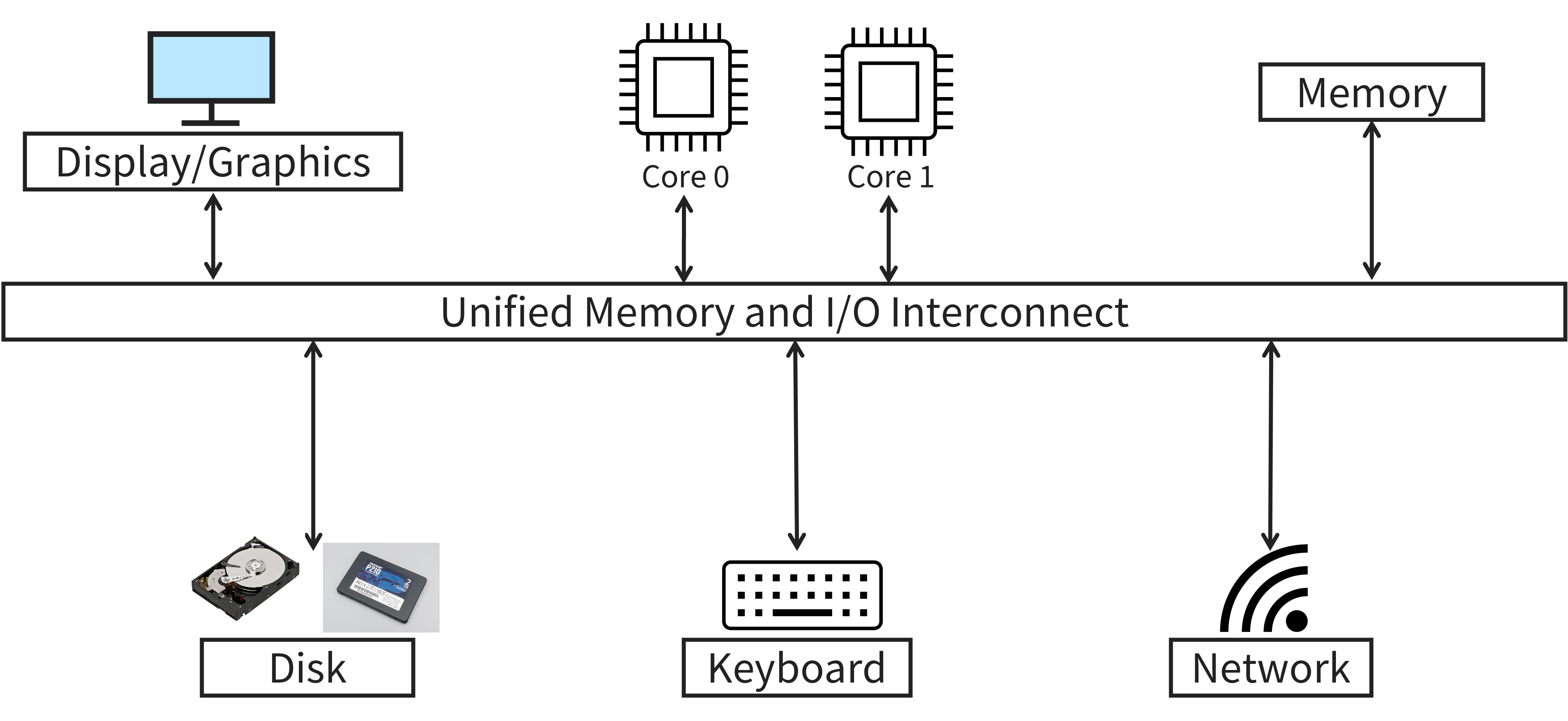
Perhaps unsurprisingly, there are several issues with this design:
-
The CPU is directly responsible for transferring data between devices. For example, suppose we want to read a file stored on an SSD and load its contents into main memory. Currently, the CPU has to communicate with the SSD over the shared interconnect and manually copy the data into main memory. As you might expect, this is time consuming and inefficient for the CPU to do as I/O devices are magnitudes slower than the CPU itself.
-
All devices have shared latency. Since all the devices on the computer are communicating over a shared channel, all communication must happen at the same speed too! Think back to the highway analogy: most highways have a speed limit. It would be rather dangerous to have some vehicles going 100 mph while others go 5 mph1! As a result, the slowest device determines how fast the interconnect can be, meaning that main memory and your keyboard would transfer data at the same rate.
-
If the interconnect were to change (e.g., it broke, desire to upgrade), all devices would need to be replaced. The physical connection interface, the interconnect latency, and/or the communication protocol are all device specific. There is no guarantee that the new interconnect would be backwards compatible with the old interconnect. This is clearly wasteful and undesirable.
Attempt 2: I/O Controllers
One of the key downsides of our first attempt was that our I/O devices were directly connected to the unified interconnect, requiring the CPU to manage each I/O device. Additionally, if the interconnect were to change, we’d need to replace all of the devices with it. Our next iteration introduces a buffer between the I/O devices themselves and the interconnect, called an I/O controller. An updated diagram is shown below.
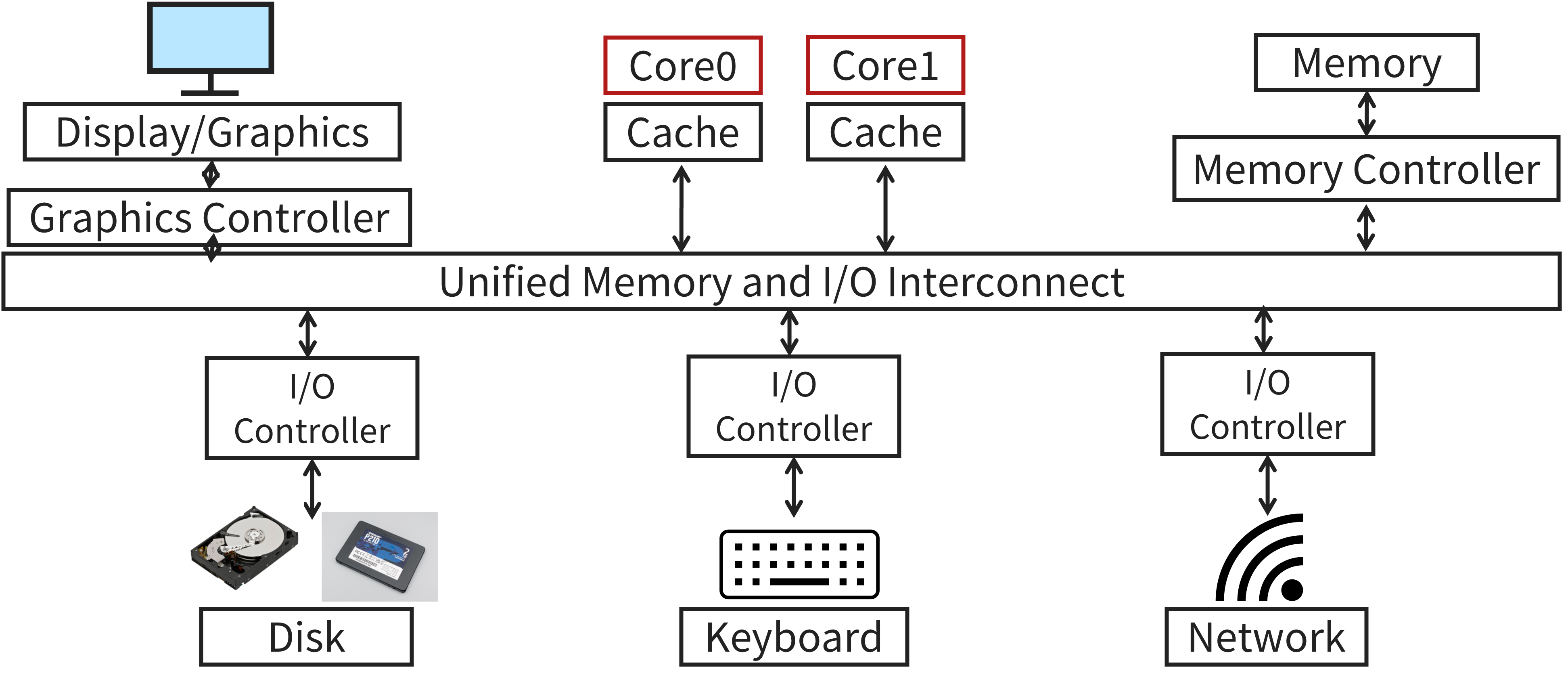
I/O controllers are responsible for managing data transfer between the CPU and the other devices connected to it. This offloads the tedious task of data transfer away from the CPU, freeing it to perform more important, compute intensive jobs. Additionally, we have removed the dependency between the interconnect and the I/O devices. If we had to change the interconnect, we could keep our I/O devices as long as the new I/O controller is compatible. Lastly, these I/O controllers can afford support more device specific features. Before, the CPU would have to know how to interact with each individual I/O device. I/O controllers abstract away many device-specific details from the CPU, decreasing cross-device dependencies. Overall, I/O controllers enable smarter, more efficient I/O interfaces.
Attempt 3: Interconnect Hierarchy
Our second attempt was a step in the right direction, but we still have the issue of shared latency to deal with. Some components, like main memory and graphics, are order of magnitude faster than lower-performance devices like storage drives and keyboards. This observation leads us to our final design, shown below.
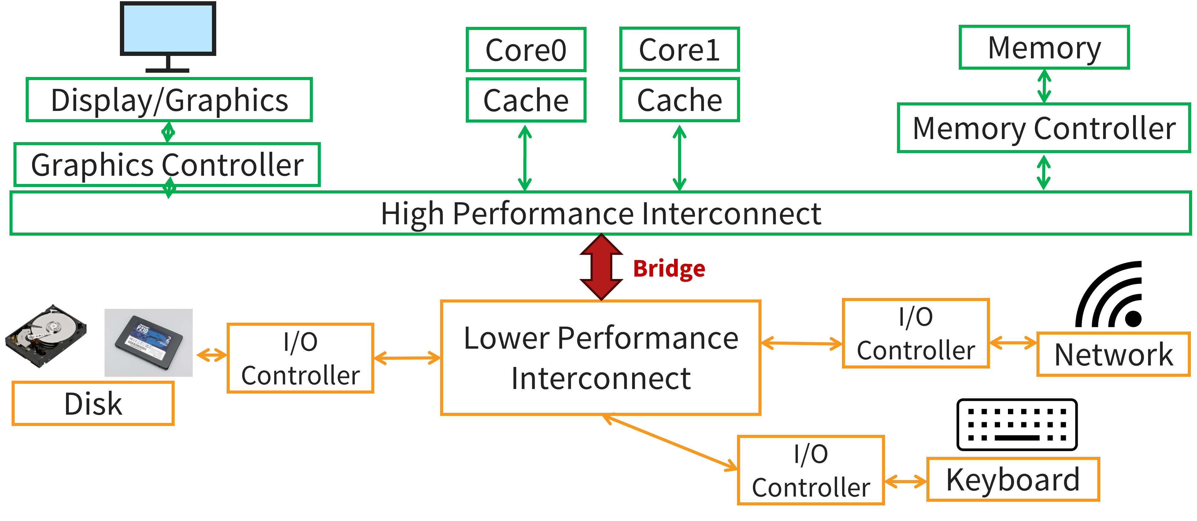
Now we have two interconnects: a high performance interconnect for high performance devices such as the CPU, graphics, and main memory, and a lower performance interconnect which connects all the other, slower I/O devices. Then, we connect these two interconnects together with a bridge. For example, Intel’s proprietary bridge is called the Direct Media Interface (DMI). The processor is still able to communicate with the I/O devices connected to the lower performance interconnect via the bridge without bottlenecking the data transfer rate between the CPU and main memory, for instance.
You might be asking why we need this hierarchical structure like this? The short answer is physics and cost. At the end of the day, the interconnect sends electrons across a piece of metal, which takes time. The shorter the distance the electrons need to travel, the faster the data transfer is. Additionally, engineering a high performance interconnect is quite costly. Therefore, it is desirable to put components that demand high performance nearer to the CPU and lower performance components further away. Another benefit of this construction is that since you can place the slower devices further away from the CPU, you have more space to connect these devices, and so you can connect more of them to a single interconnect.
The high performance interconnect, often called the “front side bus” or the “North side bus”, is short, fast, and wide (think more lanes in a highway). Consequently, the lower performance interconnect, or the “South side bus”, is longer, slower, and narrower. The upside is that they have a more flexible topology to allow for more (and more varied) connections. Not only is this construction more efficient, it is more usable as the dependency between the core of the computer (e.g., the CPU, memory, graphics) from the peripherals (e.g., USB thumbdrive, mouse, keyboard, SSD).
Examples
Recall that an interconnect is more than just a bunch of wires; the communication protocol, or bus protocol, is equally important. Further, as we’ve established, in order to handle the diverse array of I/O devices at our disposal, we need a range of hierarchical interconnects.
Perhaps the most widely known interconnect is the Universal Serial Bus (USB), geared towards connecting a wide range of external peripheral devices. SATA and SCSI are used to connect storage devices. Faster devices, such as NICs, usually use PCIe (Peripheral Component Interconnect Express). Modern SSDs are increasingly use the NVMe specification on top of PCIe to support faster storage devices. Graphics cards also use PCIe, but usually with many more parallel lanes than other PCIe compatible devices like NICs.
Modern datacenters also employ point-to-point (direct) interconnects which connect whole computers together. For example, InfiniBand (primarily used by NVIDIA) has a throughput of up to 2400 gigabit/sec! HyperTransport can be roughly understood as AMD’s variant of InfiniBand.
I/O Device API
The canonical I/O device has two parts: the internals and the interface. Internally, modern I/O devices have a few hardware chips (perhaps even a simple CPU) to implement the abstraction that the device presents to the system. They also typically have a bit of memory. Firmware is the software the runs on these internal chips that implements its functionality.
The second part of all I/O devices is the interface. Typically, there are a set of read-only and/or read/write registers that are split into three categories: the status registers, which can be read to query the status of the device, the command registers, which can be written to tell the device to do something (e.g., write data, perform a self test), and the data registers, which are used to transfer data between the device and the rest of the computer.
For example, the IBM PC/AT’s keyboard has four, one-byte registers: a status register, a command register, an input register, and an output register.
The status register is broken up further into eight flags, each a single bit.
The least significant bit of the status register, for instance, is set to 1 when the output register is full and 0 when it is empty.
This keyboard supports a number of commands, such as performing a self test.
To do this, we just have to write the byte 0xAE to the command register.
Once the test is done, we can read the result from the output register.
Accessing I/O Device Registers
There are two ways of interacting with I/O devices.
The first is called programmed I/O (PIO).
PIO is simple; we have our main CPU execute special instructions to transfer data to/from the I/O device.
The inb/outb system call functions allow us to read/write a single byte from/to a given port.
A port is simply a name for the device register we want to access represented as an integer, defined by the device.
These instructions are usually privileged, meaning the OS is in charge of who gets to access the devices.
Let’s write a function which reads the character that was just pressed using the PIO method.
char read_kbd() {
char status;
// Wait until key has been pressed
do {
sleep();
// Read status register
status = inb(0x64);
} while (!(status & 2));
// Return the character that the user entered from the input register
return inb(0x60);
}
The read_kbd() function returns the character that was most recently entered on the keyboard.
First, the OS waits for a key to be pressed by repeatedly reading the status register and checking whether the IBF flag is set, indicating that the input register is full.
This is called polling.
The second method of interacting with I/O devices is known as memory mapped I/O. This approach makes the I/O device’s registers available as if they were memory locations. To access a particular register, we can either load or store from that memory address. The hardware then routes the load/store to the device instead of main memory.
struct kbd {
char status, pad[3];
char data, pad[3];
};
char read_kbd() {
kbd *k = mmap(...);
char status;
do {
sleep();
status = k->status;
} while (!(status & 2));
return k->data;
}
Notice that the structure of the memory mapped version of read_kdb() is nearly identical to the PIO version.
We still are polling the device to know when a key has been pressed.
However, instead of making explicit calls to inb(), we mmap() the registers into the kbd struct.
Then, to access these registers, we just need to load/store from/to the status and data fields.
The hardware forwards these loads/stores to the I/O device for us.
Memory mapped I/O is popular because it allows us to depict the structure of the I/O device’s interface in software by defining a struct.
With PIO, we not only need these special inb() and outb() system calls, but we also need to know the magic port numbers that correspond to the registers we want.
Memory mapped I/O also allows us to reuse the same load/store instructions we use to access main memory.
Polling vs. Interrupts
Above, we used polling to query the status of the I/O device. While this approach is simple and it works, it feels inefficient as we are putting the CPU to sleep while it waits for data to be ready. It would be great if we could instead have the OS issue a request to the I/O device, put the calling process to sleep, and then context switch to another task while we wait. Luckily, we have already seen the perfect mechanism to implement this behavior: interrupts. Using interrupts, we can have the I/O device inform the CPU when it is done fulfilling a request. Interrupts allow us to perform computation and I/O in parallel.
It is worth noting though that interrupt-based I/O is not always more efficient than polling. If the device is fast, the cost of interrupt handling and context switching may exceed the time spent sleeping in polling. For this reason, interrupts tend to make more sense for slow devices. Many systems use a hybrid approach that polls for a little while and then, if the device hasn’t finished yet, falls back to using interrupts.
Direct Memory Access (DMA)
While interrupts allow us to avoid polling, we still have a pretty glaring inefficiency that we need to handle. Suppose we are using PIO to transfer a large amount of data to the device. Here, the CPU is stuck with the tedious task of copying data from main memory to the device. Ideally, we want our CPU to work on difficult, compute intensive tasks and not mundane ones.
To solve this inefficiency, we introduce Direct Memory Access (DMA). A DMA controller is a specific device whose sole purpose is to transfer data between main memory and I/O devices on behalf of the CPU. The CPU is then free to work on other, more pressing jobs while DMA handles the trivial task of data transfer.
To use DMA, first the CPU sends a DMA request telling the DMA controller where the data lives in memory, how much data to copy, and which device to send it to. Once the request is sent, the CPU is free to work on anything else while the DMA controller works on fulfilling the request. Once completed, the controller raises a hardware interrupt, informing the CPU that the transfer is complete. The key benefit of this approach is that the CPU is no longer stuck being the middle-man between the I/O device and main memory. DMA is the technology that enables memory-mapped I/O.
Cache Coherency & DMA
Unfortunately, DMA can lead to cache coherency problems. Suppose we want to write some data to a storage drive. If the cache is not flushed to main memory before the request is sent, the drive will receive stale data. Similarly, if we read some data from the same storage drive, the cache could become stale. If we don’t invalidate the cache after the DMA controller writes the updated to memory, the CPU will operate on the stale data currently in cache.
There are two solutions: a software-based solution and a hardware-based solution. With software enforced coherence, the OS must flush the cache before an outgoing DMA transfer is started. For incoming DMA transfers, the OS must invalidate the cache lines that are affected by the transfer. The OS could also mark certain pages as “uncacheable” to prevent the issue of cache coherency from cropping up at all! Naturally, all these methods introduces some amount of overhead to each DMA request.
Hardware enforced coherence, or snooping, uses hardware to constantly monitor the transactions between the I/O devices and main memory. When the “snooper” detects a transfer from an I/O device to memory, the snooper invalidates or updates the data in cache. Similarly, the snooper also determines whether to have cache service an outgoing DMA request or RAM, depending on which memory location has the most up-to-date value.
A notable exception is the Bundesautobahn (a.k.a., the Autobahn) in Germany which is largely devoid of speed limits.
Memory Safe Languages
This semester we have emphasized the importance of memory safety. Back in our fifth lecture when we introduced The Heap Laws, we claimed that following these laws were the hardest part of programming in C. Now that you have spent nearly an entire semester programming in C, I hope you can see why! You likely dealt with frustrating segmentation faults, searched for memory leaks, and perhaps even encountered a double free or two. All of these problems result in undefined behavior, meaning that anything could happen (like demons flying out of your nose). In the best case, your program crashes because it tried to do something it shouldn’t have. In the worst case though, your program contains extremely dangerous vulnerabilities that can be nigh impossible to find.
For example, the Morris worm relied on a buffer overflow vulnerability (among others) to spread itself across the entire Internet, causing between $100,000 and $10,000,000 in total economic impact. As a fun aside, the Morris worm was written by Robert Tappan Morris during his first year of graduate school here at Cornell University! The 2024 CrowdStrike outage last July is another prominent, recent example where an out-of-bounds read prevented roughly 8.5 million Windows systems globally from booting. The worldwide economic impact of the outage has been estimated to be upwards of $10 billion. A 2019 study by Microsoft found that 70% of all the security vulnerabilities found in their software stemmed from memory safety issues. In 2020, Google reported that around 70% of all “serious security bugs are memory safety problems” in the Chromium project. Hopefully these few examples have illustrated how severe memory safety bugs can be.
Take a moment to reflect on the fact that these problems are really only possible in languages like C and C++, where the programmer (i.e., you!) is responsible for managing memory on the heap. In contrast, Python, Java, OCaml, Swift, Haskell, C#, Go, and Rust are all memory safe languages, meaning that they manage the heap automatically for you. This is not just a convenience; these languages can rule out out these extremely dangerous memory bugs altogether. As we will shortly see, while they give up some performance or control to do so, programmers in these languages find these downside to be an acceptable trade-off to avoid the extreme challenge posed by memory bugs. The rest of this lecture focuses on how these languages automatically manage dynamically allocated memory for you.
Garbage Collection
Garbage collection is a popular strategy that many languages (e.g., Java) use to automatically free dynamically allocated memory. A garbage collector is a system that searches the heap for memory blocks that were allocated by the program, but are no longer used. Garbage collection was invented by John McCarthy in 1959 for the LISP programming language.
The goal of a garbage collector is to find and free all memory that is unreachable (garbage) by the program at a given point in time.
To do this, garbage collectors make the key insight that memory can be viewed as a directed graph, where the vertices are memory blocks and the edges are pointers or references between blocks.
Each vertex can have an arbitrary number of edges pointing in and pointing out.
For example, the integer 42 can have any number of pointers pointing to it, but because 42 is a value, not a reference, it wouldn’t have any outgoing edges.
On the other hand, a struct or a Java object may have any number of incoming and outgoing edges.
The graph may also contain cycles and self-loops.
Tracing Garbage Collection
The most common type of garbage collector is known as a tracing garbage collector. Usually when people refer to garbage collection, they are talking about tracing garbage collection. These garbage collectors employ a two-phase algorithm called mark-and-sweep to locate unreachable memory. In the mark phase all reachable memory is marked as, well, reachable. Then, in the sweep phase all memory that has not been marked as reachable is freed. Let’s take a closer look at each phase in turn.
The mark phase is concerned with figuring out which memory blocks are reachable. Informally, a block is reachable if there a pointer to it or it is otherwise accessible. For example, we can assume that local and global variables are always accessible by the program. We call the set of memory blocks that we assume are always reachable the root set. We can now formally define reachability:
A memory block is reachable if it is either:
- in the root set, or
- referenced (pointed) by a block of memory that is reachable.
Tri-Color Marking
This definition of reachability essentially outlines how the mark phase distinguishes reachable memory blocks from unreachable ones. First, the garbage collector builds the directed graph of memory. Then, it uses some tree-traversal algorithm (such as DFS or BFS) to find all the vertices starting at the root set. While traversing the graph, the garbage collector colors each vertex it touches one of three colors: white, grey, and black. The first time the collector visits a memory block, it colors it as grey. Grey denotes the vertices which are reachable, but whose edges haven’t yet been fully explored. You can think of the grey vertices as a sort of “worklist” for the garbage collector. Once all the outgoing edges of a vertex has been explored, the vertex becomes black. Black vertices are fully explored, reachable memory blocks. All the remaining, unreachable memory blocks are left white. The mark phase terminates when all grey vertices have been exhausted.
At this point, all vertices in the graph are either black or white. The sweep phase then goes through the entire heap and frees all white memory blocks.
Example
Let’s see an example of a mark-and-sweep garbage collector in action! Below is a graph of all memory blocks that currently exist in a program. There are two root nodes on the left-hand side (e.g., local variables).

The first step is to color the root nodes grey.

Next, the garbage collector explores all of the outgoing edges from all of the grey vertices until all the grey nodes have been exhausted.

The last step is for the garbage collector to dispose of all the garbage (i.e., the white vertices).

Reference Counting
Another popular strategy of automatic memory management is reference counting. In comparison to the mark-and-sweep algorithm, reference counting is pretty simple! Instead of periodically searching for unreachable memory, reference counting keeps a tally of how many references (e.g., pointers) each memory block has. Whenever a new reference is created, the tally is incremented. Similarly, when a reference is deleted the tally is decremented. When the tally reaches zero (i.e., there are no references/pointers pointing at the memory block), the object is freed.
Example
Let’s work through an example together. Consider the graph below depicting the layout of memory at some point in a program.

Square boxes around a “P” denote local pointer variables. Vertices A-H are memory blocks located on the heap. Take a moment to count how may references currently exist for memory blocks A-H. Once you’ve given it a go, you may check your answer below.

Now suppose that the reference inside of memory block A currently pointing at memory block B is updated to point to memory block G, shown below in red.

By updating this pointer, a reference to G was created and a reference to B was destroyed. So, memory block G’s reference tally is incremented to 2 and memory block B’s tally is decremented to 0 (shown below).

Since B’s tally is now zero, its memory is freed. However, by doing so one of C’s incoming references has been destroyed! Whenever a memory block is freed, reference counting recursively updates the tallies of all memory blocks that were referenced by the freed memory block. So, memory block C’s tally is decremented to 1, as shown below in red.

At this point, all the reference counts are updated and all memory blocks with a tally of 0 have been freed. However, we have a problem: memory blocks C-E are unreachable from the rest of the program’s memory but they haven’t been freed. Worse, they will never be freed, resulting in a memory leak. This example highlights the key disadvantage of reference counting: it is unable to handle cycles. Because memory blocks C-E form a cycle, their reference counts will never drop below 1. Therefore, their memory will never be freed. For this reason, languages that use reference counting (e.g., Python) often also use a garbage collector to deal with cycles.
Garbage Collecting vs. Reference Counting
We just discussed one of the key downsides of reference counting over garbage collection, namely that reference counting struggles with cyclical references. Garbage collection avoids this issue by directly checking whether each node is reachable from the root set.
Another key distinction between these two techniques is when each are run. Garbage collection is run periodically; it can run when memory is low, when it is manually triggered, or simply on a schedule. However, when it runs it must pause execution of the program. If it didn’t, the program might modify the edges of the memory graph while the garbage collector is traversing the graph. This could result in memory errors as the garbage collector might inadvertently free memory that was just made reachable. As you might expect, pausing the program to run garbage collection can have significant performance impacts. It can also be difficult or impossible to predict when garbage collection may run, causing issues for timing-sensitive programs. In comparison, reference counting updates tallies as soon as a pointer is created or destroyed. While this still affects performance, the benefit is that memory is freed as soon as it is no longer referenced.
Garbage collection and reference counting also differ in the amount of metadata each must manage. Garbage collection only needs to store the “color” of each object while it is running; this mark can be as small as a single bit. Reference counting, on the other hand, needs to store a tally (i.e., an integer) for every object.
The last difference I’ll highlight is that reference counting is much simpler to to implement than garbage collection. There are many, many variations of the naive mark-and-sweep algorithm discussed above. Further, it can be easier to estimate the performance impacts of reference counting over garbage collection as reference counting more predictable. Ultimately, the choice between these two methods depends on the specific needs and constraints of the application, balancing the trade-offs between implementation complexity, performance, and memory management efficiency.
Rust
Up until now we have been discussing strategies for automatically managing memory at runtime. Dynamic, automated memory management techniques, such as garbage collection and referencing counting, generally introduce a non-trivial amount of overhead which can negatively affect performance. For example, in 2017 [one paper][pereira2017] measured the energy efficiency of many popular programming languages, from C/C++ to Python and Java. They found that C was the most energy efficient language, primarily because C doesn’t have the overhead that (most) memory safe languages do. The one exception to this rule is Rust.
Rust is a strongly typed, compiled, memory safe, systems-oriented programming language first released in 2012.
Rust’s killer feature is that memory is managed at compile-time rather than runtime.
That is, the compiler knows where to insert de-allocation calls (i.e., free()).
This results in the best of both worlds — a memory safe language without the runtime performance impacts of garbage collection and/or reference counting!
Additionally, now that undefined behavior is caught at compile-time rather than runtime, Rust programs also tend to exhibit greater reliability and stability over C/C++ programs.
There is no such thing as a free lunch, though. Rust requires the programmer to follow certain ownership rules. These rules — which are checked by the compiler — encourage memory-safe programming and allow the compiler to accurately determine where to allocate and deallocate memory.
Ownership
Ownership is Rust’s “secret sauce” for how it efficiently manages memory at compile-time. In Rust, all data has a single owner in the form of a variable. Only the data’s owner can access it. Then, when the variable goes out of scope the memory associated with the variable is deallocated. Let’s see a few examples.
fn increment(x: i32) -> i32 { x + 1 } fn main() { let n = 5; let y = increment(n); println!("The value of y is: {y}"); }
The program above is simple: it initializes the variable n with the value 5, calls increment() with the argument n which just returns n+1, and prints this value out.
A few notes:
- All memory in this program is stored on the stack, just like in C.
- In Rust, if the last line of a function’s body doesn’t end in a semicolon, the expression is implicitly returned. So, the
increment()function’s body could also be written asreturn x + 1. - An
i32is a signed, 32-bit integer. In comparison, au32is an unsigned, 32-bit integer.
Let’s trace the ownership of the value 5.
First, 5 belongs to the variable n.
Next, when increment(n) is called, ownership is transferred or moved to the variable x in the increment() function.
Then, when the function returns, ownership is moved to the variable y.
Lastly, ownership is moved for a final time when the println! macro is called.
Now let’s see an example with dynamic memory allocation on the heap.
fn make_and_drop() { let a_box = Box::new(5); } fn main() { let a_num = 4; make_and_drop(); }
In Rust, a Box is a type that allocates memory for and stores the value it is given on the heap.
So, Box::new(5) allocates memory for an integer on the heap and stores the value 5 in it.
The owner of this heap data is the variable a_box.
However, notice that a_box is local variable in the make_and_drop() function.
When the make_and_drop() function exits, a_box goes out of scope and the Box containing 5 is deallocated (or dropped, in Rust terminology).
Therefore, all the make_and_drop() function does is allocate some memory on the heap, place a value there, and then frees that memory.
Many other data types in Rust are also stored on the stack, for instance Strings.
fn greet(mut name: String) -> String { name.insert_str(0, "Hi, "); name.push_str("!"); name } fn main() { let name = String::from("Zach"); let greeting = greet(name); println!("{}", greeting); println!("Bye, {name}!"); }
The above program is a bit more complicated, so let’s step through it together.
First, name is initialized to the String "Zach".
In Rust, a String is a mutable string stored on the heap.
This String is then given as the argument to the greet() function.
The greet() function then modifies name by inserting the prefix "Hi, " and the suffix "!" before returning the updated String.
Lastly, the program prints the (just created) greeting and says goodbye to the user.
When the main() function exits, the memory associated with name and greeting are deallocated.
This is what would happen if the above program was accepted by the Rust compiler.
Unfortunately for us, Rust would reject this program as it is not memory safe.
Recall that a String is mutable, meaning we can insert and remove characters and that it is stored on the heap.
When "Hi, " is inserted at the beginning of name, more memory might have to be allocated for name.
In fact, if this were to happen, a fresh, larger memory block would first be allocated, the old data would then be copied into the new memory block, and lastly the old memory block would be freed.
This means that the data that name was pointing to back in the main() function may no longer exist (i.e., name could be a dangling pointer).
So, Rust would return a compiler error flagging the last line of the above program.
To fix this, we need to keep the data associated with name separate from the data that we provide to the greet() function.
There are many ways to do this, but one simple way is to clone the data.
The program below does just that and will be accepted by Rust’s compiler.
fn greet(mut name: String) -> String { name.insert_str(0, "Hi, "); name.push_str("!"); name } fn main() { let name = String::from("Zach"); let name_clone = name.clone(); let greeting = greet(name_clone); println!("{}", greeting); println!("Bye, {name}!"); }
References
While cloning data is a quick and easy fix, it is inefficient.
Ideally, we would like to reuse name, but Rust’s ownership rules won’t let us.
This is where references come in.
A reference is a non-owning pointer. References allow us to provide temporary access to a variable without transferring ownership. For example, the program below uses references — denoted with an ampersand — to print the same strings as before.
fn greet(name: &String) { println!("Hi, {name}!"); } fn main() { let name = String::from("Zach"); greet(&name); println!("Bye, {name}!"); }
Now when we call greet() we pass it &name instead of name.
Similar to C, by prefixing name with an ampersand we are creating a reference to name.
Since references don’t own the data they point to, we don’t get an error when we say goodbye to the user.
However, there is a catch. In Rust, all variables and references are all either immutable or explicitly marked as mutable. Immutable references are aliases to some data. They cannot be used to write or in any way modify the data they point to. Mutable references, on the other hand, can read or write to the data they point to. Still, neither own the data they point to.
To prevent memory errors, Rust restricts how many references there can be to a single piece of data. Specifically, in any scope there can be either:
- any number of immutable references, or
- at most one mutable reference referring to the same variable. It is the job of Rust’s borrow checker to enforce these rules.
Rust Resources
Hopefully this quick introduction to Rust has piqued your interest enough to learn more! If so, here are some handy resources to start with:
- The Rust Programming Language is the official, free, online textbook for Rust. It is the best place to get started learning Rust.
- The Rust website contains many links to other learning resources and instructions for installing Rust.
- The Rust playground is an online Rust environment that you can use to play around with small Rust programs. For example, here is a link to a playground with the code from earlier!
- Rust by Example provides many examples of all the major features of Rust. It can be helpful to quickly get a feel for the language.
Lab 1: Nice 2 C You
View the lab slides here.
Before coming to lab, go through the course setup materials for Git and the RISC-V Infrastructure. The lab tasks will assume you have at least set up your Cornell GitHub credentials and have your favorite text editor, such as Visual Studio Code, ready to go.
Step 1: Group Work
Welcome to CS 3410! For the first activity of this lab, the TAs will review some of the topics from the first couple of lectures and lead a group activity. Then, you will complete a worksheet with your groups before moving on to setting up your course Docker container and completing a short coding exercise.
There’s no digital material for this part. The TAs will provide the worksheet after the review and icebreaker.
Step 2: Compiling and running C programs
Course Docker Container
Follow these instructions to set up Docker and obtain CS 3410’s Docker container. To summarize, you will need to:
- Install Docker itself.
- Download the image with
docker pull ghcr.io/sampsyo/cs3410-infra. - Consider setting up an
rvalias to make the container easy to use.
If you don’t already have a favorite text editor, now would also be a good time to install VSCode.
C Programming
Next, follow these instructions for writing, compiling, and running your first C program.
When your program runs, show the result to a TA. Congratulations! You’re now a C programmer.
Git
Now, we’ll get some experience with Git! If you haven’t already, be sure to follow our guide to setting up your credentials on GitHub so you have an SSH key in place.
Go to the to the Cornell GitHub website and create a repository called “lab1”. This repository can be public, but for assignments all of your repositories must be private.
Next, clone your repository from within a preferred directory on your device:
git clone git@github.coecis.cornell.edu:netid/lab1.git
Make sure to replace netid with your actual NetID. If this doesn’t work, ask a TA for
assistance. There is probably something wrong with your GitHub configuration.
Before changing directories into the
repo, you should move your hi.c file that you created during the Docker setup step into the lab1 folder and clean up the executables
we made earlier:
mv hi.c lab1
rm a.out
cd lab1
ls
If you haven’t created hi.c or a lab1 folder yet, you can run:
mkdir lab1
cd lab1
printf '#include <stdio.h>\nint main() { printf("hi!\\n"); }\n' > hi.c
You should see the file hi.c in your repository. Enter:
git status
The following should appear (or something like it):
On branch main
No commits yet
Untracked files:
(use "git add <file>..." to include in what will be committed)
hi.c
Now, you should add the file hi.c to stage it, make a commit, and then
push to the remote repository:
git add hi.c
git commit -m "Initial commit"
git push
This is commonly the GitHub workflow for a single person working on an assignment. You’ll make some changes, commit them, and push them, over and over until you finish the assignment.
To learn more about Git, consider following our complete git tutorial!
Step 3: print_digit and print_string
For this next task, you are going to write two helper functions to help you in Assignment 1:
print_digit(int digit): Given an integerdigitbetween 0 and 15, printdigitas a hexadecimal digit using lowercase letters to the terminal (without usingprintf)print_string(char* s): Given a string, print it to the terminal (without usingprintf)
First, cd into your lab1 repository. Then, make a file called lab1.c, and
copy/paste the following code:
#include <stdio.h>
// LAB TASK: Implement print_digit
void print_digit(int digit) {
}
// LAB TASK: Implement print_string
void print_string(char* s) {
}
int main(int argc, char* argv[]) {
printf("print_digit test: \n"); // Not to use this in A1
for (int i = 0; i < 16; ++i) {
print_digit(i);
fputc(' ', stdout);
}
printf("\nprint_string test: \n"); // Not to use this in A1
char* str = "Hello, 3410\n";
print_string(str);
return 0;
}
Save the file and exit the editor. Now is a good time to commit and push your changes to your repository. Once you’ve pushed, try to implement the functions print_digit and print_string. The TAs are available for help should you need it. A good starting point should be to look into the fputc function:
fputc (defined in stdio.h) writes a single character to a given output
stream (e.g., stdout). See more here.
For print_digit, you’ll want to use an ASCII table.
Once you’ve implemented the functions, you can run the program:
rv gcc -Wall -Wextra -Wpedantic -Wshadow -std=c17 -o test_lab1 lab1.c
rv qemu test_lab1
Like many commands on this page, this assumes you have the rv aliases setup as described in our RISC-V Infrastructure setup guide.
Remember, if you change lab1.c between runs, you need to recompile the program using the first of the commands above.
At this point, you should check off with a TA so they can check your work. Congrats! You’ve just finished your first lab in CS 3410.
Lab 2: Minifloat
You will work on a two part worksheet. Please attend the section you are registered for to receive your lab checkoff.
Lab 3: Dynamic Memory & Linked Lists
You will complete three problems on a worksheet, followed by an implementation of a singly-linked list. Please attend the section you are registered for to receive your lab checkoff.
For this week’s lab work, there are three files:
In the first part of the lab, you will review basic concepts of C memory management, completing the three worksheet problems to reinforce your understanding as you go along.
In the second half of the lab, we will introduce the implementation of a singly-linked list. Your job here is to commplete the code in lab3.c, specifically:
Node *list_create(void *a_value): Create a list containing a node of pointer toa_value.Node *list_push_to_front(Node *a_head, void *a_value): Add a new node with valuea_valueto the front of the list.Node *list_pop_last(Node *a_head): Detach and return the last node of the list.void list_free(Node *a_head): Deallocates the entire linked list.
Of these, the trickiest one is probably list_free, in which you must deallocate an entire linked list. Don’t forget to also deallocate each list node’s value!
You can test your code with an invocation of our container and only two lines:
rv
gcc -Wall -Wpedantic -Wshadow -std=c17 -o test_lab3 lab3.c
qemu test_lab3
Lab 4: C Review & GDB
In this lab, you will complete a C review worksheet and debug a C program, sel_sort.c, using ASan and GDB. Links to the lab slides, the worksheet, and material for the debugging exercise are provided below. Please attend the section you are registered for to receive your lab checkoff.
Lab 5: CPU Simulator
You will work on a three part worksheet. Please attend the section you are registered for to receive your lab checkoff.
Lab Slides
Worksheet
RISC-V ISA Reference
RISC-V Instruction Handout
RISC-V IInstruction Set Manual
Lab 6: Assembly
You will work on a worksheet that will develop your skills translating C to RISC-V assembly. Please attend the section you are registered for to receive your lab checkoff.
Lab 7: Assembly Functions
You will complete some problems on a worksheet, followed by an implementation of recursive summation function. Please attend the section you are registered for to receive your lab checkoff.
For this week’s lab work, there are three files:
In the first part of the lab, you will review RISC-V Assembly and Calling Conventions concepts, completing the three worksheet problems to reinforce your understanding as you go along.
In the second half of the lab, we will write a recursive function that sums the integers from 1 through n.
The function we want to implement would look something like this in C:
int sum(int n) {
if (n == 0)
return n;
return n + sum(n - 1);
}
In assembly, recursive function calls work exactly the same way as any other function call—the caller and callee just happen to be the same function. We’ll follow the RISC-V calling conventions in both roles.
Start by writing the function body.
The interesting part is implementing the function call.
Take note of which caller-saved registers you need to save before the jal instruction and restore after the function returns.
Next, write the prologue and epilogue.
You’ll want to start by making a list of all the values this function will ever need to store in its stack frame.
Determine the stack frame layout, or the offsets you’ll store each value at.
Lastly, follow the recipe from the add_one step in the lab slides to write the prologue and epilogue.
Copy the RISC-V assembly of the recsum function above into a file called recsum.s.
Trying It Out: Calling Your Function From C
We can’t run this assembly program yet as it lacks a main function.
It also doesn’t print anything out, which makes it hard to tell what it’s doing (if anything).
One way to test your assembly functions is to write a C program that calls your assembly function.
Make sure that your recsum.s implementation has an recsum: label.
Now, at the top of the file add the following line:
.global recsum
This directive .global tells the assembler that the recsum label is a global symbol, meaning it’s accessible to other code.
We have provided a main function you can use to test your code in recsum.c
That recsum declaration is called a prototype header, which means it doesn’t have a function body.
It just tells the C compiler that the function is implemented elsewhere—in your case, in an assembly file.
Now, let’s compile and link these two files together.
$ rv gcc recsum.s recsum.c -o recsum
Then, to run the program use rv qemu recsum n, where n is the integer to perform the recursive sum on.
This works thanks to the magic of calling conventions! You and GCC are both “assembly programmers”, and because you agree on the standard way to invoke functions, the assembly code you both write can interoperate.
Lab 8: Buffer Overflow
You will work on a worksheet that will prepare you for your buffer overflow assignment. Please attend the section you are registered for to receive your lab checkoff.
Lab 9: Cache Simulator
You will work on a worksheet that will prepare you for your cache simulator assignment. Please attend the section you are registered for to receive your lab checkoff.
Lab 10: Shall
You will work on a worksheet that will prepare you for your shall assignment. Please attend the section you are registered for to receive your lab checkoff.
In the first part of the lab, you will complete two implementation tasks.
- Invoke the
killsystem call without using standard library wrappers. - Implement a signal handler for
SIGSEGVthat recovers from segmentation faults.
In the second part, you will review system calls that will be useful for your upcoming Shall assignment.
Part 1
As you recall from lecture, processes run in an “restricted environment” called the user space. On their own, processes can run computation instructions and access its own memory. However, it cannot directly perform privileged operations such as reading files, creating processes, or writing to files. To request such privileged operations, a process must use system calls, which transfer control to the operating system kernel to perform the requested action safely on its behalf.
In this part of the lab, you will learn how the kill system call works and use it to send signals between processes.
System Calls
Signals are a way for processes to communicate with each other and notify each other of events. For example, when you press Ctrl+C in the terminal, a SIGINT signal is sent to the foreground process to interrupt it. For this exercise, we will write a function called void send_sigint(int pid) that sends a SIGINT signal to the process with the given PID.
Step 1 Learn more about kill
In rv-debug, run the following commands to see how the kill system call is defined by the linux kernel.
cat /usr/include/asm-generic/unistd.h | grep __NR_killcat /usr/include/signal.h| grep kill
You should find that the kill system call is assigned the number 129 and has 2 arguments: process id and signal to send.
Step 2 Write the send_sigint function in RISC-V assembly.
# in send_sigint.s
.global send_sigint
send_sigint:
# the first argument, pid, is already in the correct place (a0)
# the second argument, SIGINT, is 2, and must be stored in the a1 register
addi a1, x0, 2
# load the syscall number for kill (129) into a7
# - write the correct line below
# - for the answer, scroll to bottom of the webpage and reference hint 1
#### BEGIN TODO ####
### END TODO ###
ecall
ret
You can use the assembly above from C code by writing a function declaration for it
// in send_sigint.c
extern void send_sigint(int pid);
int my_atoi(const char *s) {
int n=0, sign=1;
if(*s=='-'||*s=='+') sign=(*s++=='-')?-1:1;
while(*s>='0'&&*s<='9') n=n*10+(*s++-'0');
return sign*n;
}
int main(int argc, char* argv[]) {
if (argc < 2) return 0;
send_sigint(my_atoi(argv[1]));
return 0;
}
Step 3 Compile and run the program.
Ensure you are in the rv-debug docker container. To compile, run
root@1ab8790910e4:~/test# gcc -o send_sigint send_sigint.s send_sigint.c
In a second terminal, run docker exec -it testing /usr/bin/env bash and spawn a new python process
root@1ab8790910e4:~# python3
Python 3.10.12 (main, Sep 11 2024, 15:47:36) [GCC 11.4.0] on linux
Type "help", "copyright", "credits" or "license" for more information.
>>> import os
>>> os.getpid()
378
If we run qemu ./send_sigint 378, replacing 378 with the PID that you see, we can see that the python process is will print keyboard interrupt. The program you wrote sent a signal to another process without importing any headers!
Exception Handling (OPTIONAL)
An exception is an event that occurs during the execution of a program which disrupts the normal flow of instructions. Examples include division by zero, or references to invalid memory. When an exception occurs, the CPU stops executing the current instruction and transfers control to the operating system. From there, the OS can choose to handle the exception (for example, page faults), or report it to the user program using signals (for example, SEGV for segmentation faults (invalid memory access)).
In this brief example, we will write a program that will handle the SEGV signal. The signal handler will skip over the instruction that caused the exception and continue executing the program!
The following code will abort due to a segmentation fault. Please compile with gcc -O0. Try it out! (don’t forget to use qemu)
volatile int *pointer = 0x0;
int main(void) {
*pointer = 42;
return 0;
}
Now let’s add some code which registers a signal handler for SIGSEGV. The signal handler will modify the program’s context to skip over the instruction that caused the segmentation fault.
#include <stdio.h>
#include <signal.h>
#include <stdlib.h>
void segv_handler(int sig, siginfo_t *info, void *ctx_void) {
// pointer to context that will be resumed when this context returns
ucontext_t *ctx = (ucontext_t*)ctx_void;
greg_t pc = ctx->uc_mcontext.__gregs[REG_PC];
// NOTE: please don't ever do this in a real program. This is RISC-V specific
// and relies on undefined behavior, which is why we must use "-O0"
// modify the saved program counter so that when we return from this handler,
// execution continues *after* the faulting instruction
ctx->uc_mcontext.__gregs[REG_PC] = pc + 4;
printf("Caught SIGSEGV at PC = 0x%lx (fault address = %p)\n", (long)pc, info->si_addr);
}
volatile int *pointer = 0x0;
int main(void) {
// register the signal handler
struct sigaction sa;
sa.sa_sigaction = segv_handler;
sa.sa_flags = SA_SIGINFO;
sigemptyset(&sa.sa_mask);
sigaction(SIGSEGV, &sa, NULL);
// original, problematic code
*pointer = 42;
printf("I'm still alive\n");
return 0;
}
When you run this program, it will catch the segmentation fault, skip over the offending instruction, and print “I’m still alive”.
Hints
addi a7, x0, 129
Lab 10.5: Optional Review
Lab this week will be an optional review of topics covered after the midterm (RISC-V calling convention, caches, virtual memory).
We will have a worksheet and work through solutions together. It will NOT be open office hours like the previous optional lab. However, we will not take attendance, so there is no obligation to attend (but we strongly encourage it!).
Lab 11: Concurrent Hash Table
You will work on a worksheet that will prepare you for your concurrent hash table assignment. Please attend the section you are registered for to receive your lab checkoff.
Lab 12: Parallel Raycasting
You will work on a worksheet that will prepare you for your concurrent hash table assignment. Please attend the section you are registered for to receive your lab checkoff.
A1: Implementing printf
Instructions: Remember, all assignments in CS 3410 are individual. You must submit work that is 100% your own. Remember to ask for help from the CS 3410 staff in office hours or on Ed! If you discuss the assignment with anyone else, be careful not to share your actual work.
The assignment is due via Gradescope at 11:59pm on the due date indicated on the schedule.
Submission Requirements
You will submit your completed solution to this assignment to Gradescope. You must submit:
my_printf.c, which will be modified with your solution for Task 1 and Task 2test_my_printf.c, which will contain your tests for your solution for Task 1 and Task 2
Restrictions
- You may not include any libraries beyond what is already included in
my_printf.h - Your solution should use constant space (you should not use arrays, either dynamically or statically)
- You may add as many helper functions as you would like in
my_printf.c(including those you wrote in Lab 1!), but you must leave the function signatures formy_printfandprint_integerunchanged. You may not changemy_printf.h, as we will be using our own header file for grading.
Provided Files
The provided release code contains four files:
my_printf.h, which is a header file that contains the required function definitions and some useful include statements. You may not modify this file. You may also not include any libraries in your implementation beyond what is already included in this file.my_printf.c, which contains the function definitions for your implementation. This is where you will write your code formy_printfandprint_integer.test_my_printf.c, which is a test file with a couple test cases to get you started. You must add more tests to receive full credit for this assignment.test_my_printf.txt, which is a text file that you can use to compare your outputs to by “diff” testing. See more in Running and Testing.
Getting Started
To get started, obtain the release code by cloning the a1 repository from GitHub:
git clone git@github.coecis.cornell.edu:cs3410-2025fa-student/<YOUR NET ID>_A1.git
- Note: Please replace the
<YOUR_NET_ID>with your NetID. For example, if you NetID iszw669, then this clone statement would begit clone git@github.coecis.cornell.edu:cs3410-2025fa-student/zw669_A1.git
Overview
In this assignment you will implement your own version of printf (see the
documentation here) called
my_printf from scratch. Recall that printf works
by taking in a format string that contains various format codes, in addition
to a variable number of other arguments. The format codes specify how to “plug in”
the arguments into the format string, to get the final result. For example:
printf("I love %d!", 3410); // prints "I love 3410!"
printf("Hello, %s", "Alan"); // prints "Hello, Alan"
printf("Hello %s and %s!", "Alan", "Alonzo"); // prints "Hello Alan and Alonzo!"
You will implement two key functions:
print_integer(int n, int radix, char *prefix): Print the integerntostdoutin the specified base (radix), withprefiximmediately before the first digit.my_printf(char *format, ...): Print a format string with any format codes replaced by the respective additional arguments.
Your implementation will be contained in my_printf.c. We’ve provided you with the
function signatures to get you started. You should look at my_printf.h for detailed
function specifications.
Assignment Outline
- Task 1: You will implement the
print_integerfunction - Task 2: You will implement the
my_printffunction
Implementation
Task 1: print_integer
For Task 1 and Task 2, all your code should be in the “a1” Git repository. See the Getting Started section for how to retrieve the starter code. Your implementation will be contained in my_printf.c and test_my_printf.c.
If you would like to use the print_digit and print_string functions that you wrote in Lab 1, you should copy and paste them into my_printf.c from your lab1.c file that you implemented for Lab 1.
The print_integer function takes a number, a target base, and a prefix string and prints the
number in the target base with the prefix string immediately before the first
digit to stdout. radix may be any integer between 2 and 16 inclusive. For
values of radix above 10, use lowercase letters to represent the digits
following 9 (since bases higher than 10 canonically use lowercase letters as
well).
This function should not print a newline. Here are some examples:
print_integer(3410, 10, "")should print “3410”print_integer(-3410, 10, "")should print “-3410”print_integer(-3410, 10, "$")should print “-$3410”print_integer(3410, 16, "")should print “d52”print_integer(3410, 16, "0x")should print “0xd52”print_integer(-3410, 2, "0b")should print “0b11111111111111111111001010101110”print_integer(-3410, 16, "0x")should print “0xfffff2ae”
For the radix 10, negative numbers should be printed with a negative sign (-).
All other bases should use the 2’s complement representation from lecture. In
other words, it should not print a negative sign, and instead just print
an unsigned integer representing a 2’s complement number. This is exactly what
printf from the standard library does when you pass in negative integers for
bases other than 10. You can try this on your own:
#include <stdio.h>
int main() {
printf("-10 in hex is: %x\n", -10);
printf("-10 in binary is: %b\n", -10); // Note: requires C23
}
The above code outputs:
-10 in hex is: fffffff6
-10 in binary is: 11111111111111111111111111110110
which is the 2’s complement representation of -10 in hex and binary, respectively.
You are not allowed to call any functions from the C standard library except for fputc anywhere in your implementation.
You should print a character to the console using fputc(c, stdout), where c is the character you want to print.
Tip: In addition to the documentation on cppreference.com, you can also find documentation for many standard library functions in C through the manual pages (“manpages”) in your terminal. Simply type:
man fputc
to pull it up. You can scroll through it and then type q to exit.
You must not make any assumptions about the size of an integer on a
given platform. On our platform, an integer is 32 bits, but C allows int to
be different sizes on different platforms. For example, on some architectures
int is 64 bits. Thus, you cannot store the new representation of the integer as a string or in a buffer of any size, as this would make assumptions about how big an integer is on your platform. Calling malloc is also prohibited
(by extension of the fact that stdlib.h is prohibited). In other words, you
should figure out how to do this without using any additional memory. Additionally, other string manipulation or streaming functions are also prohibited. Some example of such functions are strcpy, strncpy, strcat, strchr, strtok, sprintf, printf.
Storing characters or integers in an array (dynamically or statically) will result in a significant deduction.
You’ll also need to figure out how to print the integer from left-to-right instead of right-to-left without using additional memory. One of the algorithms you might recall from class for changing the base of a number would give you the digits from right-to-left, so it can seem tempting to try to use this as a starting point. Be warned that this will not work, as any tricks such as “reversing” the output or storing the digits would violate the constraints of this assignment (i.e. no standard library usage and no storing values in an array). Instead, think of how you can work backwards from the methods you’ve learned in class.
Task 2: my_printf
This function prints format with any format codes replaced by the respective
additional arguments, as specified below:
Your my_printf function is required to support the following format codes:
%d: integer (int,short, orchar), expressed in decimal notation, with no prefix.%x: integer (int,short, orchar), expressed in hexadecimal notation with the prefix “0x”. Lowercase letters are used for digits beyond 9%b: integer (int,short, orchar), expressed in binary notation with the prefix “0b”.%s: string (char*)%c: character (int,short, orchar, between 0 and 127) expressed as its corresponding ASCII character%%: a single percent sign (no parameter)
For each occurrence of any of the above codes, your program shall print one of
the arguments (after the format) to my_printf(...) in the specified format.
Anything else in the format string should be expressed as is. For example, if
the format string included "%z", then "%z" would be printed. Likewise, a lone
“%” at the end of the string would also be printed as is (note that this differs
slightly from the behavior of printf).
Note that strings in C can be NULL. If my_printf is passed a null string
as an argument, it should not crash, but instead print (null) to represent the
would-be string:
#include <stdio.h>
int main(int argc, char* argv[]) {
my_printf("Null string: %s", NULL); // Prints: "Null string: (null)"
}
Again, you are not allowed to call any C standard library functions. You
should print to stdout only using fputc (documentation for fputc is here).
For any format codes relating to numbers, your program should handle any valid
int values between INT_MIN and INT_MAX, inclusive.
Note that my_printf is a variadic function, meaning it takes in a variable
number of arguments. You don’t need to know this deeply, but you will
need to look up the syntax, and also understand how a program determines the
number of arguments.
A variadic function is any function that takes in an unknown number of optional
parameters. The optional parameters are represented by three dots (e.g. int foo(int n, ...)).
The dots are a part of the C language. The optional arguments are accessed using
va_arg from stdarg.h. You must call va_start at the start of your
variadic function before the first use of va_arg. You must call va_end once
at the end of your variadic function, after the last use of va_arg. There is
no way to know from va_arg how many optional arguments there are, so you
need to use some other information to determine how many times to call va_arg.
In this case, it is the format string. Here’s an example from the GNU
documentation:
#include <stdarg.h>
#include <stdio.h>
int add_em_up(int count,...) {
va_list ap;
va_start (ap, count); /* Initialize the argument list. */
int sum = 0;
for (int i = 0; i < count; i++)
sum += va_arg (ap, int); /* Get the next argument value. */
va_end (ap); /* Clean up. */
return sum;
}
int main(int argc, char* argv[]) {
/* This call prints 16. */
printf("%d\n", add_em_up (3, 5, 5, 6));
/* This call prints 55. */
printf("%d\n", add_em_up (10, 1, 2, 3, 4, 5, 6, 7, 8, 9, 10));
return 0;
}
Here are some examples to help you understand the spec:
my_printf("3410")should print “3410”my_printf("My favorite class is %d", 3410)should print “My favorite class is 3410”my_printf("%d in hex is %x", 3410, 3410)should print “3410 in hex is 0xd52”my_printf("The pass rate in 3410 is 100%%")should print “The pass rate in 3410 is 100%”my_printf("Professor %s and Professor %s are the instructors", "Weatherspoon", "Susag")should print “Professor Weatherspoon and Professor Susag are the instructors”
Note that insufficient parameters could lead to undefined behavior (i.e. when the number of arguments is less than the number of format codes). You do not have to handle this case. Similarly, mismatched parameters (when the format code does not match the given argument’s type) can also lead to undefined behavior, but you do not need to handle this.
You are encouraged to use print_integer in my_printf.
Nonetheless, these functions will be tested independently.
Running and Testing
Like many commands on this page, this assumes you have the rv aliases setup as described in our RISC-V Infrastructure setup guide.
To compile your code, run:
rv gcc -Wall -Wextra -Wpedantic -Wshadow -std=c17 -o test_my_printf test_my_printf.c my_printf.c
Then, to run your code:
rv qemu test_my_printf
We will be testing your code by comparing the output of your program to a test
file. You will extend the file test_my_printf.txt with your own
test cases. You are required to write more tests, and the quality of the tests
will be graded. Feel free to use the examples in this handout as a starting
point.
To receive full credit for testing, you should have at least 10 test cases
each for print_integer and my_printf. Test cases should cover as many
paths through your code as possible. To receive full credit for testing for print_integer,
you should have at least:
- One test representing integers for each base from 2-16
- One or more tests for different prefixes
- One or more tests with no prefixes
To receive full credit for testing my_printf you should have at least:
- One test for each format code
- One test for no format codes
- One test that contains multiple format codes
To compare the output of your program with the test file, run:
rv qemu test_my_printf > out.txt && diff out.txt test_my_printf.txt
If you don’t see any output from this command, your tests are passing. Note,
for each test you add in test_my_printf.txt, you must call the corresponding
function (either print_integer or my_printf) in test_my_printf.c. You
should insert newlines between your test cases for readability. You may use
printf in your test file, if you wish.
Don’t forget to recompile your code between different runs of your program.
Note, you can do this all in one command, like such:
rv gcc -Wall -Wextra -Wpedantic -Wshadow -std=c17 -o test_my_printf test_my_printf.c my_printf.c && \
rv qemu test_my_printf > out.txt && \
diff out.txt test_my_printf.txt
Submission
Submit my_printf.c and test_my_printf.c to Gradescope.
Upon submission, we will provide a smoke test to ensure your code compiles and passes the public test cases.
You are also required to fill in the AI survey form to mark your submission as completed. You can find the survey as a separate assignment from Assignment 1 on Gradescope.
Rubric
- 40 points:
print_integercorrectness - 50 points:
my_printfcorrectness - 10 points: test quality
- 0 points: survey
A2: Minifloat
Instructions: Remember, all assignments in CS 3410 are individual. You must submit work that is 100% your own. Remember to ask for help from the CS 3410 staff in office hours or on Ed! If you discuss the assignment with anyone else, be careful not to share your actual work.
The assignment is due via Gradescope at 11:59pm on the due date indicated on the schedule.
Submission Requirements
For this assignment, you will need to submit the following five files:
minifloat.c, with your written implementation for the missing functions.minifloat_test_part1.expected, to match additional tests added inminifloat_test_part1.c- Some additional tests, in:
minifloat_test_part1.cminifloat_test_part2.c
Restrictions
For this assignment, you will build your own floating-point representation.
- You may not use built-in C operations for floating-point arithmetic.
- You may not cast data to
floatordouble, or create variables with these types.
Provided Files
The provided release code contains seven files:
minifloat.c, which includes some completed functions and some functions you are expected to implementminifloat.h, which provides declarations and comments for the functions inminifloat.c, including those you are to implementminifloat_test_part1.c,minifloat_test_part2.cwhich provide some tests for you to get started. You are expected to add more tests of your own to each of these test suitesminifloat_test_part1.expected, which provides a baseline file to help with testing part 1. You are expected to add more lines to this file as part of testing part 1.Makefile, which provides structure to compile your code (see our brief tutorial on Makefiles)
Getting Started
To get started, obtain the release code by cloning your assignment repository from GitHub:
git clone git@github.coecis.cornell.edu:cs3410-2025fa-student/<NETID>_A2.git
Replace <NETID> with your NetID. For example, if your NetID is zw669, then this clone statement would be git clone git@github.coecis.cornell.edu:cs3410-2025fa-student/zw669_A2.git
Overview
In this assignment, you will develop a custom minifloat data format in C. You will be expected to reason about floating-point details and implement operations over your custom floating-point data type in C.
Background
In class, we learned about floating-point numbers, which represent decimals with some number of bits.
C has built-in float and double types, which use (on modern hardware)
32 bits and 64 bits, respectively.
Increasing the number of bits in a floating-point representation gives it more precision and more dynamic range, at the expense of less efficient arithmetic.
It can also be useful, however, to perform operations with smaller floating-point representations—trading off precision for potentially faster calculations.
In this assignment, you will implement functions for a specialized 8-bit floating-point type. We’ll call these 8-bit numbers minifloats. Minifloats have severely limited precision, but such tiny floating-point values are useful for situations where errors matter less and data sizes are enormous: most prominently, in machine learning. See, for example, this paper and this other paper that both show serious efficiency advantages from using 8-bit minifloats. While most floating-point formats enjoy built-in hardware support, we can also implement minifloats in software with bit packing tricks.
Minifloats follow a similar representation strategy to the standard IEEE floating-point types that we learned about in lecture. However, they differ in a few important ways to make the implementation simpler, which we will summarize as well.
Minifloat Specification
- Minifloats use 8 bits in total: 1 sign bit, 3 exponent bits, and 4 significand bits. The layout of a minifloat looks like this, with
sfor sign,efor exponent, andgfor significand:
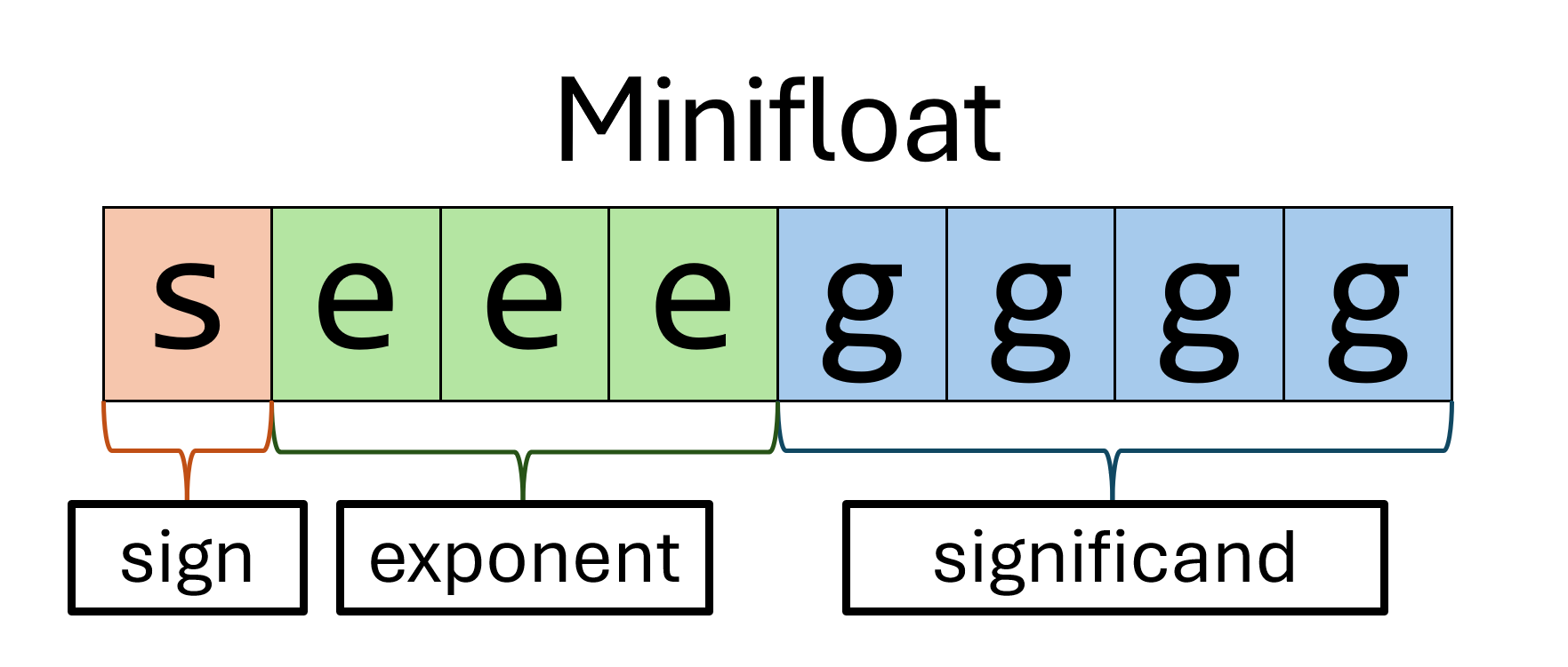
-
As in standard formats, a sign bit of
0indicates a positive number, and a sign bit of1indicates a negative number. -
Minifloats have a bias of 3. In other words, we subtract 3 from the bit-representation of a minifloat exponent. In comparison, single-precision floating-point numbers (i.e.,
float) have a bias of 127. -
Unlike standard floating-point formats, wherein we usually append a leading 1 to the significand bits with the \(1.g\) notation, minifloats use the significand directly, with the binary point after the first digit. So if the four significand bits are \(g_3 g_2 g_1 g_0\), then the “base” part of the represented value is the binary number \(g_3 . g_2 g_1 g_0\). Or, in other words, the value is \(g \times 2^{-3}\), where \(g\) is the unsigned integer value of those 4 bits.
-
Also unlike standard floating-point formats, our minifloats do not use special values: not a number (NaN) and infinity (+∞ and -∞).
All together, the value represented by a minifloat with sign \(s\), exponent \(e\), and significand \(g\) is:
\[ (-1)^s \times (g \times 2^{-3}) \times 2^{e - 3} \]
Or, equivalently, if you prefer to think of the significand’s representation in terms of bits:
\[ (-1)^s \times (g_3.g_2g_1g_0) \times 2^{e - 3} \]
where \(g_3\) is the significand’s most significant bit, \(g_0\) is the least significant bit, and so on.
Examples
Now that we have defined our minifloat specification, let’s see some examples!
Example 1: 10111100
We have a sign of 1, an exponent of 011, and a signficand of 1100.
- Our sign bit
1corresponds to \(-1\). - Our exponent
011corresponds to a decimal exponent of \(3-3 = 0\). (We’re applying our \(-3\) bias here.) - Our significand
1100corresponds to the decimal \(12 \times 2^{-3}=\frac{12}{8}=1.5\). (Or, equivalently, the significand corresponds to the binary number \(1.100_2\), which is \(1.5\) in decimal.)
Altogether, 10111100 is \(-1 \times 1.5 \times 2^0 = -1 \times 1.5 \times 1 =
-1.5\) in base-10.
Example 2: 00010010
We have a sign of 0, an exponent of 001, and a significand of 0010.
- Our sign
0corresponds to \(+1\). - Our exponent
001corresponds to a decimal exponent of \(1-3 = -2\). - Our significand
0010corresponds indicates the binary value \(0.010_{2}\), which equals \(0.25_{10}\).
Altogether, 00010010 is \(1 \times 0.25 \times 2^{-2} = \frac{1}{16} =
0.0625\) in base-10.
Converting between Minifloats and Decimals
Decimal to Minifloat
To convert a decimal number into a minifloat:
- Convert the integer and fractional parts into binary.
- Normalize to match the format \( g_3.g_2g_1g_0 \times 2^e \).
- Convert exponent into biased form (i.e., add 3).
- Set the sign bit accordingly.
Example: Converting 2.25 into an 8-bit float
Step 1: Convert the integer and fractional parts to binary.
Converting the integer portion into binary yields 10.
Our fractional part is 0.25. To convert, multiply the fractional part by 2, record the integer part of the result (should be 0 or 1), and repeat with the new fractional part until the fractional part becomes 0 or the precision limit is reached (is 4 digits for our minifloat format). The recorded integer parts of this process becomes our binary representation for the original fractional part.
- \( 0.25 \times 2 = 0.50 \). Record
0. - \( 0.50 \times 2 = 1.00 \). Record
1.
Thus our binary representation of 0.25 is 01. Together with the integer
portion, our binary representation of 2.25 is 10.01.
Step 2: Normalize to match the format \( g_3.g_2g_1g_0 \times 2^e \).
Now we normalize our result so that it fits the format \(g_3.g_2g_1g_0 \times
2^e\). In this case, we shift to the left by one place: \(1.001 \times
2^1\). From this we can see that our significand is 1001.
Step 3: Convert exponent into biased form (i.e., add 3).
Next, we need to apply our format’s exponent bias, which for minifloats is 3. To
bias the exponent, we add our original exponent \(e\) with the bias. So,
\(1 + 3 = 4\) (100 in binary).
Step 4: Set the sign bit accordingly.
Lastly, because 2.25 is positive, the sign bit should be set to 0.
Thus the minifloat representation of 2.25 is 01001001.
Minifloat to Decimal
To convert from a floating-point number into a decimal number:
- Extract the sign, exponent, and significand.
- Normalize the significand to the format \( g_3.g_2g_1g_0 \) and remove trailing zeros.
- De-normalize to make the exponent 0.
- Convert the integer and fractional parts to decimals.
- Add a negative sign if necessary.
Example: Converting 11011100 into a Decimal
Step 1: Extract the sign, exponent, and significand.
- Sign bit:
1(negative) - Exponent:
101 - Significand:
1100
Step 2: Normalize the significand to the format \( g_3.g_2g_1g_0 \) and remove trailing zeros.
Our significand 1100 becomes 1.1.
Step 3: De-normalize to make the exponent 0.
We first convert our binary exponent 101 into base-10, yielding 5. We then
subtract our bias (which is 3 for minifloats) from our exponent to get \( 5-3=2 \).
Since our exponent is 2, we shift our binary point 2 places to the right, yielding 110.0.
Step 4: Convert the integer and fractional parts to decimals
Next, we convert the integer and fractional parts of 110.0 into base-10. Since \(110_2 = 6_{10}\) and \(0_2 = 0_{10}\), \(110.0_{2} = 6.0_{10}\).
Step 5: Set the sign according to sign bit
Since the sign bit is 1, the final value is: \(-6.0\).
Adding Minifloats
To perform addition with floating-point numbers:
- Rewrite the smaller number so that the exponents are equal, and adjust the mantissa of the number with the smaller exponent by shifting it to the right accordingly.
- Add the mantissas together.
- Recombine and renormalize the result if necessary.
Example: \(1.5 + 0.5\)
First, we need to convert 1.5 and 0.5 into their minifloat representations. For 1.5 this is \(1.1 \times 2^0\), and for 0.5 this is \(1.0 \times 2^{-1}\).
Step 1: Adjust the mantissa
Because the exponents differ, we shift 0.5’s mantissa to the right by one: \( 1.0 \rightarrow 0.10 \)
Now both numbers have an exponent of 0.
Step 2: Add the mantissas together.
- \( 1.1_2 + 0.10_2 = 10.0_2\)
Step 3: Recombine and renormalize the result if necessary
- \( 10.0_2 \times 2^0 = 1.0 \times 2^1 \)
Thus the answer is 0 100 1000 which is equivalent to 2.0 in base-10.
Bit size in C
We want to ensure that the type we are using to represent a minifloat is exactly 8 bits.
We will use the uint8_t type from C’s stdint.h header.
(We will avoid char, even though char is 8 bits on most platforms, because C unhelpfully does not guarantee that is is exactly 8 bits everywhere.)
To break down this type’s, the uint means that bit-level operations are as on an unsigned integer, the 8 means that we expect operations to be on 8 bits, and _t is a common naming convention that indicates that this is a type.
The stdint.h header defines many similar types, like these:
| Type | Description |
|---|---|
uint8_t | unsigned integer with 8 bits |
uint16_t | unsigned integer with 16 bits |
int8_t | signed integer with 8 bits |
Your Task
This assignment is divided into two parts: displaying minifloats as decimals, and implementing operations on minifloats. Each part will have you implementing 1–3 functions, and adding test cases to help convince yourself these functions are correct. You must add at least 4 new test cases per function to what we have provided, though you may add more.
For all of your C implementations, you may not include any constants or variables of type float, double, or long double.
You may not use C’s built-in floating-point operations, such as +, on floating-point values.
In addition, in your implementation of minifloat operations (mini_eq, mini_add, and mini_mul), any integers you use must be at most 16 bits wide. For example, 32-bit and 64-bit integers are not permitted, but you can use 8-bit and 16-bit integers, either signed or unsigned.
However, note that you can use integers of any size in your mini_print implementation.
This is not an arbitrary restriction. Using a larger float representation in your implementation will defeat the purpose of the smaller representation, which is that they are smaller and faster than “normal” floating-point types. Because of floating-point error, it is also very likely to introduce incorrect results.
We have provided a mini_to_double utility function to help you with debugging and testing. You may not use this function in any of your submitted implementations, but you may use this function for writing test cases for any of your functions.
Part 1: Lab
View the lab slides here.
Review
If you need to, look over the lecture notes on standard floating-point types to remind yourself of the basic principles. And try out float.exposed to get hands-on practice!
Read over the background above and especially the specification for minifloats. To briefly summarize the minifloat format:
- Bit 7 is the sign bit
- Bits 6–4 are the exponent bits
- Bits 3–0 are the fraction bits
(Bits are numbered from the right, so 0 is the least significant bit.)
Displaying Minifloats
In this lab, your task is to implement a function for displaying minifloats in C, named print_mini. This function takes in a minifloat and must print the sign, whole number, and fractional part associated with this minifloat as a base-10 value. The exact specification, with examples, is given in minifloat.h. Your implementation should be filled into minifloat.c.
To make your task somewhat easier, we have written a concrete call to printf at the end of the each function that you may use as a guide for what to implement. Note that print_mini requires that we write 6 decimal digits—the provided printf specifier %06d will fill any integer to have preceding zeros such that the printed integer has 6 digits. To provide two concrete examples:
printf("%06d", 123)will print000123printf("%06d", 100000)will print100000
Remember, you may not include any constants or variables of type float, double, or long double, and you may not use any floating-point operations.
You may, however, use any integer arithmetic operation (including integer division and modulus).
In C, dividing two integers with i / j produces an integer.
But be sure not to include a double constant (such as 1.0) by accident.
You may find it useful to observe that \(1/64=0.015625\), and that, with integer division, \(1000000 / 64 = 15625\).
Testing Part 1
A test script to help guide your development can be found in minifloat_test_part1.c. You can build this test with the following command:
rv make part1
To test this code, you must execute the resulting .out file and pipe your print results to a file, such as with the following command:
rv qemu minifloat_test_part1.out > minifloat_test_part1.txt
Reminder: use the rv aliases for each command if you have it set up!
Finally, you must compare the resulting prints to our expected results using diff:
diff minifloat_test_part1.txt minifloat_test_part1.expected
If you observe any differences between the two, a printing test failed.
You can also combine these operations into a single bash command:
rv make part1 && rv qemu minifloat_test_part1.out > minifloat_test_part1.txt && diff minifloat_test_part1.txt minifloat_test_part1.expected
Reminder: You must add 4 new printing tests (which means modifying both minifloat_test_part1.c and minifloat_test_part1.expected).
Part 2: Minifloat Operations
Your second task is to implement an equality check, addition, and multiplication between minifloats. Specifically, you will be implementing mini_eq, and a minifloat operation of your choice:mini_add or mini_mul, both of which take in two minifloats and produce a new minifloat. As before, the specifications for each function can be found in minifloat.h, and your implementation should be written in minifloat.c.
The results of the arithmetic operation mini_add or mini_mul must produce the minifloat value closest to adding together the corresponding real numbers. If there are two possible closest real numbers, your implementation must correspond to the closest real number further from zero than the result of addition. For example, we would round 2.125 to 2.25, and similarly -1.0625 to -1.125.
If there are multiple possible minifloat representations of the resulting real number, you must return the minifloat with the smallest exponent. For example, the minifloat value 0 011 0010 could be equivalently represented as 0 001 1000, and only the latter is considered correct for these arithmetic operations. Additionally, if an arithmetic operation would return 0, you must return exactly 00000000.
If applying addition or multiplication would result in a real number larger or smaller than can be represented by a minifloat, the result of these operations is undefined, and need not be tested.
Hint: If you become stuck on any of these functions, consider attempting another—each requires detail that can become more obvious while working on another. Your grade in this part will be determined by the operation (mini_add or mini_mul) that performs more correctly.
Testing Part 2
Testing minifloat operations is more straightforward than testing the printing implemented earlier. We can simply run each test file and compare the resulting minifloats to expected values. To test part 2, you can directly build and execute part2:
rv make part2 && rv qemu minifloat_test_part2.out
Reminder: You must add 4 new tests per function. Specifically, 4 for mini_eq and 4 for either mini_add or mini_mul, the operation you chose to implement.
Hint: Write as many edge-case tests as you can think of, there are many potential tricks with negative numbers and very small or very large minifloats.
The mini_to_double utility is only for testing.
Do not use it in your main implementation.
Remember that your goal is to implement minifloat operations from scratch, using only integer arithmetic.
This is what makes minifloats more efficient than float or double.
Your tests should not include cases where the minifloat arithmetic would overflow (produce a result larger than the maximum minifloat or smaller than the largest negative minifloat). We do not define the results of these overflowing operations.
Submission
Submit minifloat.c, minifloat_test_part1.expected, minifloat_test_part1.c, and minifloat_test_part2.c to Gradescope.
Upon submission, we will provide a smoke test to ensure your code compiles and passes the public test cases.
You are also required to fill in the AI survey form to mark your submission as completed. You can find the survey as a separate assignment from Assignment 2 on [Gradescope].
Run smoke Test locally
You can build smoke test locally with the following command:
rv make smoke_test
To test this code, you must execute the resulting .out file and pipe your print results to a file, such as with the following command:
rv qemu minifloat_smoke_test.out > minifloat_smoke_test.txt
Finally, you must compare the resulting prints to our expected results using diff:
diff minifloat_smoke_test.txt minifloat_smoke_test.expected
If you observe any differences between the two, a printing test failed.
You can also combine these operations into a single bash command:
rv make smoke_test && rv qemu minifloat_smoke_test.out > minifloat_smoke_test.txt && diff minifloat_smoke_test.txt minifloat_smoke_test.expected
Rubric
- 20 points:
print_minicorrectness - 22 points:
mini_eqcorrectness - 40 points:
mini_addormini_mulcorrectness - 18 points: test quality
- 0 point: survey
A3: Huffman Compression
Instructions: Remember, all assignments in CS 3410 are individual. You must submit work that is 100% your own. Remember to ask for help from the CS 3410 staff in office hours or on Ed! If you discuss the assignment with anyone else, be careful not to share your actual work.
The assignment is due via Gradescope at 11:59pm on the due date indicated on the schedule.
Submission Requirements
You will submit your completed solution to this assignment on Gradescope. You must submit:
priority_queue.c, which will contain part of your work for Task 1.huffman.c, which will contain part of your work for Task 1 and the whole of Task 2.
Restrictions
- You may not modify any files other than
huffman.candpriority_queue.c(i.e., the files you will submit) except the test files (read the section below).
Provided Files
priority_queue.h, which is a header file that defines the specification for the priority queue.priority_queue.c, which will contain your implementation of a priority queue and stack. You will modify this file.huffman.h, which is a header file that defines the types and functions you will need to implement Huffman compression.huffman.c, which will contain your implementation for the Huffman compression system. You will also modify this one.bit_tools.h, which is a header file that defines theBitWriterandBitReaderstructs and their respective functions for reading and writing binary values from files.bit_tools.c, which contains the implementation of the functions forBitWriterandBitReader.memcheck.h, which is a header file that defines themy_mallocandmy_freemacros and their respective wrapper implementation (my_malloc_implandmy_free_impl) for allocating and deallocating memory from and to the heap.memcheck.c, which contains the implementation of the wrapper functions formy_malloc_implandmy_free_implalongside any helper functions.utils.h, which contains utility functions for printing lists and tree nodes.utils.c, which contains the implementation for the utility functions.decode_bits.py, which contains the implementation for a script to decode a coding table into a more human-readable representation.check_memory_leaks.py, which contains the implementation for a script to analyze memory allocation/deallocation logs and report memory leaks, if any.Makefile, which contains the build tools for this assignment.test_priority_queue.c, which contains all necessary functions to test your implementation for the priority queue. You may add tests here, but you will not turn this file in.test_huffman.c, which contains functions to test your implementation for Task 1. You may also modify this file (highly recommended specifically), but will not turn this file in.cu_unit.h, which contains the macro definitions that you’ll use for unit testing.compress.c, which contains the compression program’s command line interface.decompress.c, which contains the decompression program’s command line interface.
Getting Started
To get started, obtain the release code by cloning your assignment repository from GitHub:
git clone git@github.coecis.cornell.edu:cs3410-2025fa-student/<NETID>_huffman.git
Replace <NETID> with your NetID. All the letters in your NetID should be in lowercase.
Overview
In this assignment you will implement a data compression system using Huffman coding. Huffman compression is an encoding scheme that uses fewer bits to encode more frequently appearing characters and more bits to encode less frequently appearing characters. It is used by ZIP files, among many other things. The high-level overview of the algorithm is:
- Calculate the frequency of each character in the data. (Task 1)
- Build a Huffman tree using the frequencies, leveraging a priority queue. (Task 1)
- Build an encoding table using the Huffman tree. (Task 2)
- Encode each character in the data using your encoding table. (Task 2)
In task 1, you will implement a priority queue in C. You’ll use this to build your Huffman tree. The bulk of the work for this assignment will come from understanding the Huffman coding algorithm and manipulating data structures in C using pointers. There are plenty of resources on the internet (including YouTube) to help in understanding Huffman encoding. We find this video to be the quickest way to understand it in a way that’s to-the-point and easy to translate into the assignment.
Huffman Compression Algorithm
Your implementation will read a single text file as input and produce two output files: a compressed data file and a coding table file that encodes enough information to allow decompression. (This assignment does not include decompression; we have given you a decompressor implementation.) Task 2 describes the format for these files.
Before moving onto the tasks, let’s break down the Huffman compression algorithm. You may recall that ASCII is a straightforward way to represent characters. In ASCII, every character is encoded with 8 bits (1 byte). There are 256 possible ASCII values that can be represented. This means that if we use standard ASCII encodings to represent a text file, each character in the file requires exactly 1 byte. This is inefficient, as most text streams don’t actually use all 256 possible characters. The basic idea behind Huffman encoding is as follows: use fewer bits to represent characters that occur more frequently.
For example, consider the string go go gophers.
Notice how g and o appear three times more often than the remaining letters.
It would be nice if we could construct an encoding which uses fewer bits for g and o and (possibly) more bits for the remaining characters (e.g., h, r).
That’s the goal with Huffman coding.
At the heart of Huffman coding is the Huffman tree data structure. A Huffman tree is a binary tree with characters at its leaves. Each edge in the tree corresponds to a bit: a left edge corresponds to 0 and a right edge corresponds to 1. To get the encoding for a character, follow the path from the root node to the character’s leaf node and concatenate all the corresponding bits.
Here’s a Huffman tree that contains all the characters in our string, go go gophers:
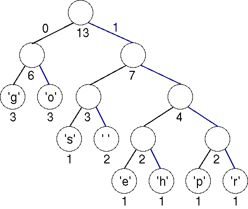
We have labeled each leaf with the frequency of that character. Internal nodes also have a frequency number that is the sum of all the frequencies of the children.
Here’s a table that shows the binary code for each character, according to this tree:
| Character | Binary code |
|---|---|
| 101 |
e | 1100 |
g | 00 |
h | 1101 |
o | 01 |
p | 1110 |
r | 1111 |
s | 100 |
Remember, you get the encoding by traversing the path from the root to the character, using a 0 for every left edge and a 1 for every right edge.
The Huffman tree ensures that characters that are more frequent in the input receive shorter encodings, and characters that are less frequent receive longer encodings. Our goal is to construct the Huffman tree, write the coding table, and write the compressed file using these shorter encodings.
Assignment Outline
- Task 1: You will implement a priority queue in C as well as the
calc_frequenciesfunction inhuffman.calongside the algorithm to create a Huffman tree. - Task 2: You will implement the functions
write_coding_tableandwrite_compressedto write the coding table and compressed bytes to distinct files.
Implementation
In this assignment, you will be allocating/deallocating memory using our wrappers my_malloc and my_free. They essentially make the same system calls (malloc and free, respectively), except that they log the operation (enabling you and us to detect any memory leaks). Do NOT use standard malloc and free in your implementation instead of my_malloc and my_free. Also, the test files will call these macros, so if your implementation doesn’t use them, there will be unavoidable memory leaks.
Task 1: Implementing a priority queue, frequency counter, and building a Huffman tree
Before starting, make sure you’ve cloned the release code by following the instructions in Getting Started.
Step 1: Implement a priority queue
The code for this portion is located in priority_queue.c, which is provided to
you in the release code. In this step, you’ll build a priority queue that accepts a “generic” data type.
This is accomplished by storing a pointer to an arbitrary piece of memory that
can store anything by using void*. We’ve provided a header
file that defines the PQNode type as well as the function declarations
for the functions you are required to implement.
Your implementation will go in priority_queue.c. We’ve provided a complete test suite
in test_priority_queue.c. You will implement the following functions:
PQNode *pq_enqueue(PQNode **a_head, void *a_value, int (*cmp_fn)(const void *, const void *)): Add a new node with valuea_valueto a priority queue, using functioncmp_fn(...)to determine the ordering of the priority queue.PQNode *pq_dequeue(PQNode **a_head): Detach and return the head. Note, the caller is responsible for freeing the detached node, and any memory it refers to. Do not callmy_free.void destroy_list(PQNode **a_head): Deallocates the priority queue. This should callmy_freeon every data element as well as the list nodes.PQNode *stack_push(PQNode **stack, void *a_value): Add a new node with valuea_valueto the front of the list.PQNode *stack_pop(PQNode **stack): Detach and return the head of the list. Note, this function is extremely similar topq_dequeue.
The last two functions are to enable us to use the same data structure as a stack,
when needed. You probably will not make use of this for your Huffman compression
system, but the decompression system needs a stack to work properly. If you can
implement pq_enqueue, and pq_dequeue, implementing stack_push and stack_pop
should be very easy.
We’ve provided a test file called test_priority_queue.c. Running rv make pqtest
from the command line will build an executable called test_priority_queue, which
you can then run by typing rv qemu test_priority_queue.
The tests use the header file cu_unit.h, which defines various macros that help
you write unit tests. In general, tests should be structured like so:
static int _test_name() {
cu_start();
//-------------------
// Setup code - build a list, declare a variable, call a function, etc.
cu_check(/*condition you want to check*/);
// ... add as many checks as you want
//-------------------
cu_end();
}
int main(int argc, char* argv[]) {
cu_start_tests(); // Indicate start of test suite
cu_run(_test_name); // Don't forget to run the test in `main`
cu_end_tests(); // Indicate end of the test suite
}
Upon running the test, you’ll see one of the two following messages:
Test passed: _test_name
which will be displayed in green, or:
Test failed: _test_name at line x
which will be printed in red, and give the line that failed. We’ve provided all the tests
you need for the priority queue (the autograder will be checking for these only).
You can add more tests to verify the functionality of your implementation, but you will not
be turning in test_priority_queue.c, however, so this will not be graded.
Generic data types
You might notice some strange looking syntax in these function declarations.
This is to enable generic data types. The PQNode struct contains a void*, which
you can think of as a memory address to any type. This allows you to use the
same code for linked lists of any type.
You can assign a void* to an address of any type. This is why you can write
code like:
char* s = malloc(...);
even though malloc(...) returns a void*, not a char*. This is also similar
to the way functions such as qsort(...) allow you to sort arrays of any type.
Just to reiterate, this is just an example - you will be using my_malloc(...)
instead in the assignment.
Function addresses
Code that deals with generic data types often needs to pass functions as parameters.
To do this, you need to specify the address to a function as an argument. In other
words, you are declaring the parameter of the function (in this case cmp_fn) as
the address to a function that takes in some parameter(s) of specified types and
returns a value of a specified type. For the compare function, you’ll always
return an integer, and the arguments to the compare function can be anything,
depending on the underlying data in the nodes of the priority queue.
Let’s look at an example:
void _print_square(int n) {
printf("%d squared is %d\n", n, n * n);
}
void _print_cube(int n) {
printf("%d cubed is %d\n", n, n * n * n);
}
void _call_print_fn(int n, void(*print_fn)(int)) {
print_fn(n);
}
int main(int argc, char* argv[]) {
_call_print_fn(4, _print_square); // Prints 16
_call_print_fn(4, _print_cube); // Prints 64
}
In the above code, the type of parameter print_fn is void(*)(int). In other
words, print_fn is the address to a function taking an int and returning void.
Generalizing this to our priority queue, notice that the type of parameter cmp_fn
is int(*)(const void*, const void*). This is the address to a function taking
two addresses to memory locations of any type and returning an int.
Implementing pq_enqueue
You might recall from CS 2110 that priority queues can be implemented with binary heaps. In our implementation, however, we will be implementing our priority queue as a linked list that we will keep sorted by priority. This means that inserting a node will be an \(O(n)\) time operation, and removing from the priority queue will be a constant time operation. This is fine for our purposes.
In pq_enqueue, *a_head refers to the head of the linked list. If
*a_head is NULL, then the list is empty. a_value is the address of whatever
value is associated with this node.
Allocate a new PQNode and insert it into the list in sorted order, according to the cmp_fn function.
Since cmp_fn(...) is a black box right now, here is how you will interpret its output.
If cmp_fn(a, b) < 0, then a is ordered before b (or a is less than b, in a sense), else otherwise.
That is, everything before the new PQNode should be less than the new one, and everything to the right should be bigger than (or equal to) the new one.
*a_head should be updated if the new node becomes the first item in the list.
The function should return the address of the new node.
This function should call my_malloc exactly once. You should not call
my_free in this function.
Implementing pq_dequeue
Like the previous function, *a_head refers to the head (first node) of a valid
linked list. If the list is empty, return NULL (since there is nothing to dequeue).
Upon return, *a_head must be a valid linked list (although possibly empty). For
our purposes, NULL is a valid linked list of size 0. Thus, *a_head will be
set to NULL if the list is empty, and upon removing the last node, you should set
*a_head to NULL.
You must also set the next field of the removed node to NULL. The caller
is responsible for freeing the detached node, and any memory it refers to.
For this reason, this function should not call my_free, directly or indirectly.
Implementing destroy_list
This function should completely destroy the linked list referred to by *a_head,
freeing any memory that was allocated for it. This function should
set the head to NULL in the caller’s stack frame (i.e. *a_head = NULL).
This is a good point to check to make sure that your code does not leak memory.
Let’s look at the following code in test_priority_queue.c:
#include "priority_queue.h"
#include "cu_unit.h"
int _cmp_int(const void *a, const void *b) {...}
void _print_int(void *a_n) {...}
static int _test_simple_pq()
{
cu_start();
// -------------------------------
PQNode *head = NULL;
int n1 = 5, n2 = 7, n3 = 6;
pq_enqueue(&head, &n1, _cmp_int);
pq_enqueue(&head, &n2, _cmp_int);
pq_enqueue(&head, &n3, _cmp_int);
cu_check(is_sorted(head, _cmp_int));
PQNode *first_node = pq_dequeue(&head);
cu_check(*((int *)first_node->a_value) == 5);
PQNode *second_node = pq_dequeue(&head);
cu_check(*((int *)second_node->a_value) == 6);
PQNode *third_node = pq_dequeue(&head);
cu_check(*((int *)third_node->a_value) == 7);
cu_check(head == NULL);
my_free(first_node);
my_free(second_node);
my_free(third_node);
// -------------------------------
cu_end();
}
int main(int argc, char* argv[]) {
cu_start_tests();
cu_run(_test_simple_pq);
cu_end_tests();
return 0;
}
This code should contain no memory leaks, i.e., it should eventually my_free everything that it my_mallocs. Note that in this case, the test case does not call destroy_list since
each list node here has a stack variable (e.g, int n1 = 5) as its element - simply invoking my_free deallocates the list node. If it were an allocated variable instead (e.g, char *c = (char *)my_malloc(sizeof(char))),
then the test case would’ve called destroy_list as it needs to deallocate both the list node as well as the allocated variable element.
Checking for memory leaks
Now is a good point to talk about how you can check for memory leaks. As mentioned above, my_malloc
and my_free log their operations to a text file memcheck_log.txt. The text file is created if it doesn’t
exist, otherwise the two wrappers keep logging operations to the text file. An operation log will look something
like this:
malloc(32) = 0x1559800b50 at huffman.c line 44
This means the following information is being logged: the operation (malloc, because that’s what’s really happening under the hood),
the bytes allocated/deallocated (32 bytes), the address in question (0x1559800b50), and the file as well as the line number where
the operation was invoked (huffman.c, line 44). We don’t expect you to sift through every address being allocated to check if
was deallocated (i.e. checking for memory leaks) as our script, check_memory_leaks.py will do that for you.
rv python3 check_memory_leaks.py memcheck_log.txt -delete
The script will read memcheck_log.txt and print a report, detailing memory leaks, if any. The -delete flag is optional, and it
deletes memcheck_log.txt after printing the report. Remember that my_malloc and my_free keep appending logs to the text file
with no understanding of which binary is being executed. In other words, if you run rv qemu test_priority_queue five times, memcheck_log.txt
will contain the operation logs of all five executions. Hence, we recommend executing a binary, reviewing its memory leak report, and deleting (or
renaming) memcheck_log.txt before the next execution so a new memcheck_log.txt file is generated and logs don’t get mixed up.
Implementing stack_push and stack_pop
In stack_push, *stack stores the address of the first node in the linked list. a_value stores
the address of the generic type. The newly allocated node should become the first node
of the list, and *stack should be updated. The function returns the address
of the new node.
In this function, you will call my_malloc exactly once, and you will
not call my_free. This function is extremely similar to pq_enqueue, except you
don’t need to think about where in the list the node should go.
It always goes in the front of the list.
For stack_pop, you should simply detach and return the node from the head
of the linked list. Note that this is incredibly similar to the specification for
pq_dequeue.
Again, make sure you thoroughly test this code, as it will be used extensively in the rest of Task 1 and Task 2. If you are confident your code is correct, now would be a good time to commit and push your work to GitHub.
Step 2: Implementing calc_frequencies
The code for this task is located in huffman.c. You will be implementing the
following function:
calc_frequencies(Frequencies freqs, const char* path, const char** a_error): Open a file atpathand either store the character frequencies infreqor set*a_errortostrerror(errno).
Before getting started, we recommend you take a look at the type definitions and function
specification located in huffman.h. In particular, pay careful attention
to these two lines:
typedef unsigned char uchar;
typedef uint64_t Frequencies[256];
The first line tell us that uchar is simply an alias for an unsigned char. Similarly,
the second line tells us that Frequencies is an alias for an array of 256 unsigned
integer values.
For the function calc_frequencies, the caller is responsible for initializing
freqs[ch] to 0 for all ch from 0 through 255. The function should behave as follows:
-
If the file is opened correctly, then set
freqs[ch]to \(n\), where \(n\) is the number of occurrences of the characterchin the file atpath. Note that acharis an integer type, so it can be used to index directly into an array. But note that, just like other integer types, we need to specify whether it is signed/unsigned.After this, return
true. Do not modifya_error. -
If the file could not be opened (i.e.,
fopenreturnedNULL), set*a_errortostrerror(errno)and returnfalse. Do not modifyfreqs.
You only need to check for errors related to failure to open the file. This
function should not print anything, nor should you call my_malloc or my_free.
You do not need them.
This function will need to use file input/output functions from the stdio.h header.
In particular, use the documentation for fopen, fgetc, and fclose.
Working with files in C can be confusing at first. Let’s look at some of the
basic syntax:
#include <stdio.h>
#include <stdlib.h>
void print_first_character(char const* path) {
FILE* stream = fopen(path, "r"); // this opens the file in reading mode
char ch = fgetc(stream); // read one character from the file, starting from the beginning
fputc(ch, stdout); // write that character to stdout
fclose(stream); // always call fclose() if you call fopen()
}
int main(int arc, char* argv[]) {
print_first_character("animal.txt");
return 0;
}
In the fopen function, the second argument indicates the mode the file should
be opened in. "r" is for reading, "w" is for writing, and "a" is for appending.
If you wanted to write a function to print out every character in a file (and
not just the first), you’d write something like this:
void cat(char const* path) {
FILE* stream = fopen(path, "r");
for (char ch = fgetc(stream); !feof(stream); ch = fgetc(stream)) {
fputc(ch, stdout);
}
fclose(stream);
}
Be sure to use the stdio.h documentation to find the I/O functions you need.
Again, we recommend testing your code for calc_frequencies before moving on.
Create a file called test_frequencies.c, and an example file such as animals.txt.
Try calling your function and seeing if it correctly obtains the frequencies of
each character in the text file using cu_unit.
Step 3: Building a Huffman tree
So far, we have created a priority queue that accepts a “generic” data type. We will use the priority queue in this task to build our Huffman tree.
The implementation for the Huffman tree will be contained in huffman.c. Look
carefully first at huffman.h to ensure you understand the functions you are
required to implement. In what remains of Task 1, you will implement these two functions:
TreeNode* make_huffman_tree(Frequencies freq): Given an arrayfreqwhich contains the frequency of each character, create a Huffman tree and return the root.void destroy_huffman_tree(TreeNode** a_root): Given the address of the root of a Huffman tree created bymake_huffman_tree(...), deallocate and destroy the tree.
Recall that freq is an array with 256 values. Each
index of the array is an ASCII character (recall that chars are just unsigned
bytes in C). The value of freq[c] is the frequency of character c in the
input file.
Also important in the header file is the definition of the TreeNode struct.
A Huffman tree node contains the character, the frequency of the character in the input, and
two child nodes. Huffman’s algorithm assumes that we’re building a single tree
from a set (or forest) of trees. Initially, all the trees have a single node
containing a character and the character’s weight. Iteratively, a new tree is
formed by picking two trees and making a new tree whose child nodes are the
roots of the two trees. The weight of the new tree is the sum of the weights of
the two sub-trees. This decreases the number of trees by one in each iteration.
The process iterates until there is only one tree left. The algorithm is as
follows:
- Begin with a forest of trees. All trees have just one node, with the weight of the tree equal to the weight of the character in the node. Characters that occur most frequently have the highest weights. Characters that occur least frequently have the smallest weights. These nodes will be the leaves of the Huffman tree that you will be building.
- Repeat this step until there is only one tree: Choose two trees with the
smallest weights; call these trees
T1andT2. Create a new tree whose root has a weight equal to the sum of the weightsT1 + T2and whose left sub-tree isT1and whose right sub-tree isT2. - The single tree left after the previous step is an optimal encoding tree.
To implement this strategy, use your priority queue to store your tree nodes. You want all the nodes to be ordered by their weights, so you can easily find the two trees with the smallest weights (at the front of the queue). You will need to write your own comparison function to implement this policy. To break ties when two tree-nodes have the same frequency, you can order them lexicographically by the ASCII value of the character.
We will not pay particular attention to the tie-breaking between a node and a non-leaf node, since those nodes are supposed to not hold a value in theory. Adding a tie-breaking here would make your implementation unnecessarily more complex. While there is only a single theoretically correct Huffman tree, this implies that the tree we build here can take on multiple forms. That’s fine; we will not grade based on the exact structure of your Huffman tree, but the properties delineated below.
When you test your code, you should make sure that calling destroy_huffman_tree(TreeNode** a_root)
ensures that your code has no memory leaks.
For testing, there are a few properties of Huffman trees we would like to verify:
- The weight of an internal node is equal to the sum of the weights of its children.
- The sum of the weights of the leaf nodes is equal to the number of characters in the uncompressed text.
- If the number of distinct leaf nodes is \(n\), then the number of total nodes in the Huffman tree is \(2n - 1\).
The last property follows from the fact that if you start with \(n\) leaf nodes, you need \(n - 1\) internal nodes to connect them.
We’ve provided you with a file test_huffman.c, which defines functions that
verify the aforementioned properties using cu_unit.h. We’ve provided three
test functions: one for each file given to you in the tests directory. You
are encouraged to add more thorough tests yourself; however, you do not need to turn
in test_huffman.c. Once you are confident your implementation is correct, move on to the next task.
To compile and run this program, you’ll run:
rv make hufftest
rv qemu test_huffman
Task 2: Writing the compressed file and coding table
Now we have all of the pieces we need to write the compressed file and
the coding table. For this task, you must implement two functions, found in huffman.c:
void write_coding_table(TreeNode* root, BitWriter* a_writer): Write the code table toa_writer->file. This function writes to a file calledcoding_table.bits.void write_compressed(TreeNode* root, BitWriter* a_writer): Write the encoded data toa_writer->file. This function writes to a file calledcompressed.bits
The above functions make use of the BitWriter struct, which is defined in
bit_tools.h. The BitWriter allows us to write data to a file in increments
of bits instead of bytes.
(Normal file writing APIs, including C’s standard stdio.h, only support writing entire bytes at a time.)
You are not responsible for fully
understanding the inner workings of BitWriter, but you do need to know how
to use it to write data to the file.
The BitWriter struct contains a file that
is already opened in "w" mode. To write bits to the file, you must call the
function write_bits(BitWriter* a_writer, uint8_t bits, uint8_t num_bits_to_write).
It takes three parameters:
a_writer: The address of aBitWriterthat contains a file which is open for writingbits: The bits you want to write, stored in auint8_tnum_bits_to_write: The number of bits you want to write, which must be between 0 and 8 inclusive
For both the compressed file and the coding table, you should only need to write
bits to the file in 1-bit and 8-bit increments. The following program may help in
understanding the behavior of the BitWriter more clearly:
int main(int argc, char* argv[]) {
BitWriter writer = open_bit_writer("new_file.bits");
write_bits(&writer, 0x05, 3); // 0x05 ↔ 00000101₂ ⋯ writes just 101₂
write_bits(&writer, 0xf3, 3); // 0xf3 ↔ 11110011₂ ⋯ writes just 011₂
write_bits(&writer, 0x01, 2); // 0x01 ↔ 00000001₂ ⋯ writes just 01₂
write_bits(&writer, 0x20, 6); // 0x20 ↔ 00100000₂ ⋯ writes just 100000₂
write_bits(&writer, 0x13, 5); // 0x13 ↔ 00010011₂ ⋯ writes just 10011₂
write_bits(&writer, 0x05, 5); // 0x05 ↔ 00000101₂ ⋯ writes just 00101₂
close_bit_writer(&writer);
return 0;
}
After running this code, you can inspect the new_file.bits file using the
following command:
xxd -b -g 1 new_file.bits
The xxd tool prints out files in binary, hex, and ASCII formats so you can see exactly what you have written.
Be careful when writing characters whose encodings are greater than 8
bits. write_bits can only write at most 8 bits at a time as bits is an 8-bit
unsigned integer (uint8_t). One way to get around this restriction is to
iteratively print the number one bit at a time. See below for an example of
how to do this:
int main(int argc, char* argv[]) {
BitWriter writer = open_bit_writer("new_file.bits");
uint32_t bits = 0x107; // 0x101 ↔ 100000111₂ --> more than 8 bits long
uint8_t num_bits_to_write = 9;
// THIS LINE WOULD FAIL because we have more than 8 bits we are trying to write in write_bits
write_bits(&writer, bits, num_bits_to_write);
// THIS LINE WORKS because we write the encoding bit-by-bit.
for(int i = 0; i < num_bits_to_write; ++i){
write_bits(&writer, bits >> (num_bits_to_write - i - 1), 1) // write the encoded bits one at a time
}
close_bit_writer(&writer);
return 0;
}
Implementing write_coding_table
The coding table is a file that encodes the structure of your Huffman tree in a
text file. It is an important utility for the decompression algorithm, as it
allows you to recover the structure of the Huffman tree without needing the original
uncompressed text. In this step, we will write the encoded Huffman tree to a file
called coding_table.bits.
To write the coding table, you do a post-order traversal of your Huffman tree.
- Traverse the left subtree of the root (i.e., encode it to the file).
- Traverse the right subtree of the root (i.e., encode it to the file).
- Visit the root.
Every time you “visit” a node (including the root of a subtree):
- If it is a leaf (i.e., character), you write one bit:
1. Then, you write the entire character (8 bits). Example: If the character isA, you will write0b101000001. The1is to signify that it is a leaf. The0b01000001is to specify the character itself. - If it is a non-leaf (i.e., an internal node), you write one bit:
0.
To write out the bits for a character, you can pass a char value directly to write_bits.
For example, use write_bits(my_writer, 'A', 8) to write out the binary encoding of the character A.
Your code will write the bits for the coding table using BitWriter. To make the coding table more explicit, consider the following Huffman tree for go go gophers again:
If we provide this tree as an input to write_coding_table, the coding table representation should look like:
1g1o01s1 01e1h01p1r0000
In complete binary (as formatted by xxd), it would be represented as:
00000000: 10110011 11011011 11010111 00111001 00000010 11001011
00000006: 01101000 01011100 00101110 01000000
Notice that the first bit is a 1, indicating a leaf, followed by the byte
01100111, which represents the character g in ASCII. Write the bits of the
coding table to the file only. Do not write anything before or after the
encoding of the Huffman tree.
Before we move on, here’s another reminder that the Huffman tree you build in make_huffman_tree can take on various forms depending on how you tiebreak the non-leaf nodes; there is no single “correct” Huffman tree for the purpose of this assignment. This means your binary representation generated by the compression driver below for go go gophers might not match the example above; in fact, in our implementation we got:
00000000: 10111001 11011001 01101101 00000101 10011101 01101111 ..m..o
00000006: 10111000 01011100 10010010 00000000 .\..
So even if your coding table for the gophers example might not match our examples in this instruction, there is no need to fret. Just make sure to verify that your coding table matches your Huffman tree and run some tests.
You can verify the functionality of your write_coding_table by running the compression driver:
rv make
rv qemu compress tests/ex.txt
xxd -b -g 1 coding_table.bits
Running the compress binary will produce two files: coding_table.bits and
compressed.bits. You can inspect each of these files to verify the correctness
of the write_coding_table and write_compressed functions, respectively.
Viewing coding_table.bits will give you the binary representation of the coding table instead
of something like 1g1o01s1 01e1h01p1r0000, which is more human-readable. If you prefer this
representation for debugging, you can using decode_bits.py to print out such a representation
of your coding_table.bits file:
rv python3 decode_bits.py coding_table.bits
Implementing write_compressed
In this step, we will write the compressed data to compressed.bits. The argument
a_writer to the function points to a BitWriter that has compressed.bits open
for writing. To write the compressed data, you will need to traverse your Huffman tree to
recover the encodings, and then use the encodings to write the compressed data.
How you accomplish this is largely up to you—there are many valid approaches
here. Just make sure that there are no memory leaks and that your compressed
data file actually represents the Huffman encodings. Again, write the bits of
the compressed data only—do not write any bits before or after the compressed
bits.
When you go to inspect the file, you may notice that there are an additional
four bytes written to compressed.bits before the compressed data itself. These
bytes represent the size of the original uncompressed text in bytes. Integers
are typically four bytes, so we use four bytes to write this information to the
file. This is written for you by the compression driver (do not write this
yourself). The reason it’s there is for decompression—the decompression
program needs to know how big the original text file was to recover the
uncompressed text.
Using the go go gophers example, the compressed data
should look something like (where there are four additional bytes at the beginning):
00000000: 00001101 00000000 00000000 00000000 01101110 11011101 ....n.
00000006: 10110000 11001011 01000000 ..@
Notice that if you use the command ls -l, you can see the sizes of your files
in the directory in bytes. The original file was 13 bytes but the compressed
file is 9 bytes—our compression was successful!
Running and Testing
To make it easier to compile and run your code, we’ve provided a Makefile. To
build your program, simply type rv make. rv make will build two executables: a
compression program and a decompression program. To run the compression
program, type:
rv qemu compress <filename>
This will produce two output files: compressed.bits and coding_table.bits. If
you run the compression program on another input file, the two output files will
be overwritten with the new results.
To run the decompression program, type:
rv qemu decompress compressed.bits coding_table.bits <uncompressed_filename>
This produces a file called <uncompressed_filename>. To see if your compression was
successful, you can try comparing the result of the decompression to the
original unencoded file by running:
diff <original_file> <uncompressed_file>
For example, if you were trying this on the cornell.txt file in the tests
directory, you’d run:
rv qemu compress tests/cornell.txt
rv qemu decompress compressed.bits coding_table.bits uncompressed_cornell.txt
diff tests/cornell.txt uncompressed_cornell.txt
If you see nothing when running this, that means the files are identical and decompressing your compressed file was successful. Good work!
Note that the decompression tool is based on your implementation of the coding table and the Huffman tree. In other words, you might be able to decompress your file correctly, but that does not mean your Huffman tree is correct.
Round-trip compression and decompression is necessary for the correctness
of the entire system, but not sufficient, to
guarantee that all of the functions from Task 1 and Task 2 are correct. You are
strongly encouraged to use cu_unit.h to more thoroughly test your code for Task 1.
You can add tests directly to test_huffman.c. You are not required to submit this file, but we strongly
encourage you to test each task separately as that is how your code will be graded.
To build the test executables, you can run:
rv make pqtest
rv make hufftest
which will generate test_priority_queue and test_huffman, respectively.
Submission Guidelines
Submit huffman.c and priority_queue.c to Gradescope. Upon
submission, we will provide a smoke test to ensure your code compiles and
passes the public test cases (including a few from test_priority_queue.c).
Since there are two weeks for this assignment, there will be two submission deadlines, one worth 15 points (due Wed 9/17) and worth 85 points (due Wed 9/24).
- For the first deadline, while we encourage implementing everything specified for Task1, you are only required to submit a working implementation of Priority Queue that is free of memory leak to qualify for the 15 points. Slip days will not be applicable on this deadline. Note that the autograder will also grade the Huffman tree implementation, but this is for those intent on implementing all of Task1 (as encouraged). Nevertheless, we will only look at the autograder’s output on priority queue tests and memory leaks to grade this submission.
- For the second deadline, you are required to submit the entire assignment. The autograder will grade the entire assignment, including the priority queue (on the same test cases as before), the Huffman tree implementation (unseen test cases included), compression/decompression (unseen test cases included), and memory leaks.
Rubric
- Submission #1: 15 points
- Submission #2: 85 points
- Priority Queue test cases: 15 points
- Huffman Tree test cases: 30 points
- Compression/Decompression test cases: 40 points
Code that contains memory leaks will be subjected to a flat 5 point deduction.
Lab 4: C Review & GDB
In this lab we will introduce two tools for debugging C code - AddressSanitizer (ASan) and the GNU Debugger (GDB). ASan is useful for catching many common memory bugs. GDB allows you to step through your code one line at a time, with the ability to see values of variables along the way.
In this lab, you a program, sel_sort.c, that contains multiple bugs. Your job is to find these bugs, using the capabilities of GDB and ASan.
ASIDE: Working with Docker + QEMU + GDB
As with other assignments in this course, you should carry out all of your work within the Docker container that is distributed as part of the course infrastructure. The combination of Docker, QEMU, and GDB appears in several real-world applications (for example, kernel debugging), so beyond the standardization it offers for our class assignments, being able to use GDB in this way will turn out to be a useful skill for you.
However, the combination of these three adds some additional complexity to the use of GDB:
-
Because it needs to work at the level of the target machine’s ISA (i.e., RISC-V), you can’t just run a compiled program directly with GDB. Instead, you will need to use GDB’s remote-connection facility.
-
The remote-connection facility requires that you have two open terminal windows: one for the executable being run under QEMU and the other for GDB to connect to that process. Unfortunately, the fact that we are running QEMU in a Docker container adds even more complication:
- Because you are running everything in a Docker container, you need to make sure that both terminal windows are invoking the exact same container instance.
Adding Debugging Support To The CS3410 Container
The CS3410 course infrastructure document suggests that you define an alias (or, on Windows, an equivalent PowerShell function):
alias rv='docker run -i --init -e NETID=<YOUR_NET_ID> --rm -v "$PWD":/root ghcr.io/sampsyo/cs3410-infra'
where <YOUR_NET_ID> should be replaced with your actual Cornell NetID.
We’ll use this as the basis for an invocation that adds two additional pieces of functionality, control of the container image’s name and support for core dumps in the current working directory:
alias rv-debug='docker run -it --rm --init -e NETID=<YOUR_NET_ID> --name testing --ulimit core=-1 --mount type=bind,source="$PWD"/,target="$PWD"/ -v "$PWD":/root ghcr.io/sampsyo/cs3410-infra'
To make the alias stick around when you open a new terminal shell, you will need to add it to your shell’s configuration file. You can do this by pasting the alias at the end of your shell’s configuration file or by typing these commands in your terminal but fill in the appropriate file according to your shell.
echo "alias rv-debug='docker run -it --rm --init -e NETID=<YOUR_NET_ID> --name testing --ulimit core=-1 --mount type=bind,source=\"\$PWD\"/,target=\"\$PWD\"/ -v \"\$PWD\":/root ghcr.io/sampsyo/cs3410-infra'" >> ~/.bashrc
As before, you don’t really need to understand the details of Docker to use this in your work, but for the curious:
-
--name testingchanges the name of the container image to “testing”, but you can choose any other name value, so long as it begins with an upper or lowercase letter. This is useful for situations in which you need to run multiple terminal windows with access to the same container image, as you will in the next section of this assignment. -
--ulimit core=-1 --mount <etc.>enables support for core dumps, which are created when a program crashes. The specific form used here ensures that a core file is always created in the current working directory.
Like rv, you can run rv-debug with zero, one, or more arguments. With zero arguments, you’ll get a bash prompt in the Docker container itself. Any arguments that are supplied are considered to be an execution of an application within the container itself.
As before, there is a similar PowerShell function that you can define if you’re working on a Windows system:
Function rv_debug {
if (($args.Count) -eq 0) {
docker run -i --init --rm -e NETID=<YOUR_NET_ID> --name testing --ulimit core=-1 --mount type=bind,source="$PWD"/,target="$PWD"/ -v ${PWD}:/root ghcr.io/sampsyo/cs3410-infra
}
else {
$app_args=""
foreach ($a in $args[1..($args.count-2)) {
$app_args = $app_args + $a + " "
}
$app_args = $app_args.Substring(0,$app_args.Length-1);
docker run -i --init --rm -e NETID=<YOUR_NET_ID> --name testing --ulimit core=-1 --mount type=bind,source="$PWD"/,target="$PWD"/ -v ${PWD}:/root ghcr.io/sampsyo/cs3410-infra $args[0] $app_args
}
}
Try adding this to the function_rv_d file in which you have already defined rv_d. As with the Linux/MacOS version, you should be able to run this just like rv_d, with or without additional arguments.
See the course infrastructure document for details on making this and the rv alias a permanent part of your working environment.
Part 1: Memory Bugs in sel_sort.c
Now that you have the aliases setup for GDB, compile sel_sort.c using the below command:
rv gcc -g -std=c23 -Wall -Werror sel_sort.c -o sel_sort
And run your code:
rv bash # Enter the interactive rv bash shell
# qemu sel_sort
Segmentation fault (core dumped)
# Your code may also hang, in that case press ^C three times in a row to exit.
Seeing the words “Segmentation fault,” “double free,” code freezing, or print statements not printing should immediately tell you to add AddressSanitizer to your code. In later assignments, approximately half of the bugs you encounter can be solved using ASan, use it!
Now add -fsanitize=address,undefined to the compile command, like so:
rv gcc -g -std=c23 -Wall -fsanitize=address,undefined -Werror sel_sort.c -o sel_sort
Running your code using qemu should give you something similar to this output:
# qemu sel_sort
sel_sort.c:28:10: runtime error: load of misaligned address 0x000000000001 for type 'long int', which requires 8 byte alignment
0x000000000001: note: pointer points here
<memory cannot be printed>
AddressSanitizer:DEADLYSIGNAL
=================================================================
==1==ERROR: AddressSanitizer: SEGV on unknown address 0x000000000001 (pc 0x000000010eec bp 0x001555d569d0 sp 0x001555d56990 T0)
==1==The signal is caused by a READ memory access.
==1==Hint: address points to the zero page.
#0 0x10eee in swap /root/sel_sort.c:28
#1 0x11182 in selection_sort /root/sel_sort.c:40
#2 0x11582 in main /root/sel_sort.c:69
#3 0x1556ace922 in __libc_start_call_main (/lib/libc.so.6+0x2b922)
#4 0x1556acea0e in __libc_start_main@GLIBC_2.27 (/lib/libc.so.6+0x2ba0e)
#5 0x10bda in _start (/root/sel_sort+0x10bda)
AddressSanitizer can not provide additional info.
SUMMARY: AddressSanitizer: SEGV /root/sel_sort.c:28 in swap
==1==ABORTING
The important line to focus on here is:
#0 0x10eee in swap /root/sel_sort.c:28
It tells us that line 28 in sel_sort.c caused the segmentation fault. Can you figure out what is wrong on line 28? ASan output can be confusing at times, if you are struggling do not be afraid to ask course staff for help.
After fixing both bugs, you might notice that your code does not print the correct output. Unfortunately, ASan cannot help find logic bugs in your code. For those, GDB is needed.
Part 2: Logic Bugs in Selection Sort
Introduction
The file sel_sort.c contains an implementation of the selection sort algorithm, with a main procedure that tests it on two different arrays. A version that passes its tests will display each array in ascending order. Sadly, it does not pass. In fact, trying to run it results in an unsorted array:
# qemu sel_sort
Test array #1:
[an unsorted array]
Test array #2:
[another unsorted array]
First, lets get GDB set up for your sel_sort.c.
Building Source Files for Debugging
In order to debug a program with GDB, you must first compile its source code with debugging symbols that allow GDB to inspect the resulting executable and display information such as program execution and variable values in terms of the original C code. To do this, compile the source file with the additional -g flag. This flag will add debugging symbols to the executable that will allow GDB to debug much more effectively.
Using GDB’s Remote Debugging
Let’s use GDB to find the bug in selection sort! Assuming you’ve already compiled sel_sort.c, open two terminal tabs or windows (a split view is recommended if your terminal app supports it):
-
In one window, start
qemuwith therv-debugalias to create a named docker container:# "-g 1234" tells qemu to wait for gdb to connect on port 1234 rv-debug qemu -g 1234 sel_sortThis will appear to hang, which is what you want.
-
In the other terminal window, run gdb inside the same container with the following docker command:
# If you changed "--name testing" to something else in the alias, use that name here docker exec -it testing gdb -q -ex 'target remote localhost:1234' -ex 'set sysroot /opt/riscv/sysroot' -ex 'set can-use-hw-watchpoints 0' sel_sortYou should see output like this:
# docker exec -it testing gdb -q -ex 'target remote localhost:1234' -ex 'set sysroot /opt/riscv/sysroot' -ex 'set can-use-hw-watchpoints 0' sel_sort Reading symbols from sel_sort... Remote debugging using localhost:1234 Reading symbols from /opt/riscv/sysroot/lib/ld-linux-riscv64-lp64d.so.1... (No debugging symbols found in /opt/riscv/sysroot/lib/ld-linux-riscv64-lp64d.so.1) 0x0000001555d6b9f4 in _start () from /opt/riscv/sysroot/lib/ld-linux-riscv64-lp64d.so.1 Reading symbols from /opt/riscv/sysroot/lib/ld-linux-riscv64-lp64d.so.1... (No debugging symbols found in /opt/riscv/sysroot/lib/ld-linux-riscv64-lp64d.so.1) (gdb)Now you have a gdb prompt and can start executing gdb commands.
GDB Basics
After you entered GDB, there are different commands you can use to help you narrow down the problems. We introduce some of them briefly in the following. With the exception of run, all of these commands should work the same way, whether you’re using GDB in our CS3410 container or natively.
Run
In the remote debugging you’ll use for this assignment and other assignments in the class, you won’t ever use this command (the qemu -g 1234 <etc.> is already running the program you’re debugging). In other settings, however, run is a fundamental part of the basic GDB toolbox. The command runs your program until a breakpoint or crash is encountered. If you are not using GDB remotely, run is the command you would type to begin execution of your program. You can also pause your program by pressing Control-C (useful for finding infinite loops). When one of these is encountered, you will be able to inspect the state of your program with any of the commands below.
Breakpoints, next, step, continue, finish
If we want to stop and see what is going on at a particular point in our program, we can use breakpoints. To
do this in GDB, type break, followed by the line number of the source code file where you want to stop. For
example, break 64 will set a breakpoint at the beginning of the main in sel_sort.c (i.e. on Line
64). If you want to set a breakpoint at the entry to a procedure, without reference to a line number, you can
type break <procedure name> instead.
If the program is already running but paused, continue will resume execution. It will stop at the next
breakpoint if there is one, and run to the end, otherwise. If you only want to run to the end of the current procedure, you can use the finish command instead.
After the program stops at a breakpoint, you can use either next or step to execute the program line
by line.
(The difference between them is that next will skip over execution of the body of a called procedure and just go to the instruction after the procedure returns, while step will pause at the first instruction of the procedure body.)
(gdb) break main
Breakpoint 1 at 0x10860: file sel_sort.c, line 60.
(gdb) continue
Continuing.
warning: Could not load shared library symbols for linux-vdso.so.1.
Do you need "set solib-search-path" or "set sysroot"?
Breakpoint 1, main (argc=1, argv=0x1555d56d18) at sel_sort.c:60
60 long test_array[5] = {1,4,2,0,3};
(gdb) continue
Continuing.
[Inferior 1 (process 9) exited normally]
If the program you are debugging closes or crashes, you will need to restart the remote debuggin process: exit GDB, restart your program with QEMU waiting on GDB, then re-launch GDB in the other terminal window.
Disable/delete breakpoints
Use the delete <N> command to delete breakpoint N, or disable <N> if you only want to disable it. It reverse, enable N , is used to enable breakpoint N. Typing either delete or disable with no arguments will delete/disable all breakpoints at once.
Backtrace
When GDB reaches an error or a breakpoint it will only tell you the line of code that it occurred on. In order to see the whole
backtrace, the whole set of stack frames associated with the file at the time, type backtrace. Use this to
find the function that called the function. sel_sort.c:<line number> tells you the file and
line number of the instruction that was running when the breakpoint was triggered.
(gdb) break swap
Breakpoint 1 at 0x106b8: file sel_sort.c, line 28.
(gdb) continue
Continuing.
Breakpoint 1, swap (a=0x1555d56b58, b=0x1555d56b70) at sel_sort.c:28
28 long tmp = *a;
(gdb) backtrace
#0 swap (a=0x1555d56b58, b=0x1555d56b70) at sel_sort.c:28
#1 0x000000000001077c in selection_sort (arr=0x1555d56b58, len=5) at sel_sort.c:40
#2 0x00000000000108c4 in main (argc=1, argv=0x1555d56d18) at sel_sort.c:69
This gives the state of the call stack and program execution point at the moment that the breakpoint was triggered. This output tells us that the last instruction to run was line 28 of a call to swap, which itself was called on line 42 of selection_sort, and so on.
While having this much information about the call stack is helpful, we will often want to have a more detailed view of what’s going on in the program. We can see the value of any variable that is in scope in the current stack frame by using the commands print and display. These instructions print the value of any expression that is semantically valid at the current line of execution; in particular, they are useful for seeing the current values of declared variables. The difference between them is that display will show the value of its expresion argument after every instruction step, while print displays it just once.
Breakpoint 1, selection_sort (arr=0x1555d56b58, len=5) at sel_sort.c:38
38 for (int i = 0; i < len; i++)
(gdb) print (i < len)
$1 = 1
(gdb) print a
No symbol "a" in current context.
(gdb) display i
1: i = 0
(gdb) step
39 int swap_idx = smallest_idx(&arr[i], len - i);
1: i = 0
(gdb) display (i < len)
2: (i < len) = 1
(gdb) s
smallest_idx (arr=0x1555d56b58, len=5) at sel_sort.c:10
10 int smallest_i = 0;
Notice how the displays fof both i and (i < len) cease when execution steps into the body of smallest_idx.
Once smallest_idx returns, the display of these expressions will resume. You can cancel an ongoing fdisplay with undisplay.
(gdb) finish
Run till exit from #0 smallest_idx (arr=0x1555d56b58, len=5) at sel_sort.c:13
0x0000000000010748 in selection_sort (arr=0x1555d56b58, len=5) at sel_sort.c:39
39 int swap_idx = smallest_idx(&arr[i], len - i);
1: i = 0
2: (i < len) = 1
Value returned is $3 = 3
(gdb) undisplay 2
(gdb) s
42 swap((long *)arr[i], (long *)arr[swap_idx]);
1: i = 0
(gdb)
Finally, a related command, x, gives a more low-level version of this same feature by showing the contents of memory at a given address. See https://visualgdb.com/gdbreference/commands/x, among other resources, for a detailed explanation.
Info
The info command provides brief summaries of important program information:
info locals—displays the values of every local variable in the current stack frameinfo args—displays the values of every parameter in the current stack frameinfo stack—displays the current call stackinfo break—displays all currently-defined breakpoints, whether they are enabled or not.
Some Advanced GDB Features
Watchpoints
Watchpoints break the program execution whenever the value of an expression changes, and the value changes will be displayed. To set a new watchpoint, you need to invoke watch with either an expression or a raw memory address. If you watch an expression, it must be semantically valid for the current execution point (i.e. all variables in scope, etc.); the watchpoint will be deleted when execution leaves the block in which the expression is meaningful. To watch the contents of a memory address regardless of the program’s block structure, use the -location (or -l) flag. For example, you could set a watchpoint on index 0 of the array test_array.
Breakpoint 1, main (argc=1, argv=0x1555d56d18) at buggy_sel_sort.c:64
64 long test_array[5] = {1,4,2,0,3};
(gdb) watch test_array[0]
Watchpoint 2: test_array[0]
(gdb) watch -location test_array[0]
Watchpoint 3: -location test_array[0]
(gdb) continue
Continuing.
Watchpoint 2: test_array[0]
Old value = 0
New value = 1
Watchpoint 3: -location test_array[0]
Old value = 0
New value = 1
0x000000000001088c in main (argc=1, argv=0x1555d56d18) at buggy_sel_sort.c:64
64 long test_array[5] = {1,4,2,0,3};
(gdb) continue
Continuing.
Watchpoint 2 deleted because the program has left the block in
which its expression is valid.
(gdb) info break
Num Type Disp Enb Address What
1 breakpoint keep y 0x000000000001086c in main at buggy_sel_sort.c:64
breakpoint already hit 1 time
3 watchpoint keep y -location test_array[0]
breakpoint already hit 1 time
4 breakpoint keep y 0x0000000000010710 in selection_sort at buggy_sel_sort.c:38
The command info break will show watchpoints as well as breakpoints. To disable a watchpoint,
type disable <watchpoint_num>.
Conditional Breakpoints
Conditional breakpoints enable you to break execution on a line of code when an expression evaluates to true.
To set a new conditional breakpoint, type break <line number> if <expression>. For example, to break from
execution when smallest_idx is not equal to arr[0] on line 17, you can type break 17 if smallest != arr[0]. Conditional breakpoints allow you to debug specific scenarios and limit the messages that you would collect otherwise when debugging without specific conditions.
(gdb) break 17 if smallest != arr[0]
Breakpoint 1 at 0x1065c: file buggy_sel_sort.c, line 17.
(gdb) continue
Continuing.
warning: Could not load shared library symbols for linux-vdso.so.1.
Do you need "set solib-search-path" or "set sysroot"?
Breakpoint 1, smallest_idx (arr=0x1555d56b58, len=5) at buggy_sel_sort.c:17
17 smallest_i = i;
(gdb) print smallest_idx
$1 = {int (long *, int)} 0x105f0 <smallest_idx>
Initialization Args & Files
Having to type target remote localhost:1234 and break 17 and continue or similar every time you want to debug a program is quite tedious. Fortunately, there are several ways to automate gdb to run commands immediately when the debugger starts: the gdb source command, -x and -ex arguments, and .gdbinit files. We actually used the -ex flag earlier!
Fix the Sorting
Now, use GDB to see what is causing your selection sort to fail.
A5: CPU Simulation
Instructions: Remember, all assignments in CS 3410 are individual. You must submit work that is 100% your own. Remember to ask for help from the CS 3410 staff in office hours or on Ed! If you discuss the assignment with anyone else, be careful not to share your actual work.
The assignment is due via Gradescope at 11:59pm on the due date indicated on the schedule.
Submission Requirements
For thsis assignment, there are two files to submit to Gradescope:
logic.cwith the listed functions all implemented.tests.txtwith all of your test cases in the correct format.
Restrictions
- You may not use any additional include directives.
- Please only change
logic.c. Changes to other files will not be reflected in your submission.
Provided Files
The following files are provided in the release:
logic.c, which includes the five functions you will implement in this assignment.runner.c, which handles I/O and the structure of the simulator.hash_table.c, an implementation of a simple hash table.hash_table.h, which is the above’s associated header file.sol.h, which includes the signatures of the functions inlogic.candhash_table.c, as well as usefuldefinemacros and variable declarations.Makefile, which will appropriately compile and link the above to produce an executable,runner.check.s, a simple assembly program to be used as a smoke test.check.bin, the input to the program, which is the result of assemblingcheck.s.
The only file among these that you will modify is logic.c.
Getting Started
To get started, obtain the release code by cloning your assignment repository from GitHub:
git clone git@github.coecis.cornell.edu:cs3410-2025fa-student/<NETID>_cpusim.git
Replace <NETID> with your NetID. All the letters in your NetID should be in lowercase.
Overview
In this assignment, you will implement a subset of the RISC-V 64 instruction set. In order to gain a better understanding of control logic, processor architecture, and how assembly language functions, you will simulate the steps—Fetch, Decode, eXecute, Memory, Writeback—of a simple single-cycle processor.
The program takes assembled RISC-V machine code into standard input. We handle the I/O and break the instructions down into an array of uint32_t values, named instructions. instructions[0] has the 32-bit encoding for the first instruction, and generally, instructions[PC / 4] has the 32-bit encoding for the PC / 4 + 1st instruction (i.e., the instruction at address PC in the input file). The instruction encodings follow the standard that is specified in the RISC-V ISA manual.
After the instructions are fed into the program, while the program counter (divided by 4) is less than the static instruction count, it will continuously, in order, call the functions fetch(), decode(), execute(), memory(), and writeback().
Each of these 5 functions passes information to the next stage. fetch() will pass the current instruction to decode(), which will pass relevant information to execute(), which will pass other information to memory(), which will pass more information to writeback(), which will update the registers and the program counter. The relevant information is stored in a struct called info, which has 4 integers. It is up to you to decide exactly what information to store in the info struct, and not every stage will need all the bits.
The info struct is meant as a container for arbitrary bits.
There is no single correct way to use its fields to represent the relevant state.
You will use the info struct in entirely different ways for each of the four stage → stage communication steps.
The 32 general-purpose registers are simulated as an array of 32 uint64_ts. The starter code initializes all of these to 0.
Memory is simulated as a hash table, data, that maps from uint64_t to uint64_t. The keys are addresses, and the values are the data stored in memory. We suggest mapping an address to one byte of data, but an alternative such as mapping addresses to four or eight bytes is also acceptable.
An implementation of a hash table is provided in hash_table.c and hash_table.h. All key (address) → value (data) mappings are effectively initialized to 0, as the ht_get() function returns 0 when the key is not found.
Use the little-endian byte order for your simulated memory.
For example, when storing an 8-byte value to address a, store the least-significant byte at a and the most-significant byte at address a+7.
Assignment Outline
- Work out a high-level plan and implement
addi,andi,ori, andxoridetailed in Task 0. - Implement the rest of the instruction subset, detailed in Task 1.
- Create a thorough test suite that you will submit, specified in Task 2.
Implementation
Task 0: Getting Started
Design Plan
As stated in the overview, one of the goals of the assignment is to familiarize yourself with the important steps in a simple five-stage processor. The figure below may be used as reference.
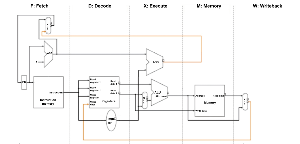
The five stages of the processor that you simulate are:
-
Fetch an instruction from main memory. The PC (Program Counter) holds the address of the instruction to fetch.
-
Decode the instruction into relevant parts that the processor understands, and read the requested register(s). Things to consider: What info is important to extract from an instruction? How should we generate the correct immediate value from the bits in the instruction? How do we single out bits that differentiate instructions—what makes
lwdifferent fromswor fromsb? -
Execute the instruction to determine its result value.
-
Access memory (here simulated as a hash table) to load/store data, if necessary. Things to consider: How should the stage differentiate bytes vs. words vs. double words? When should this stage sign-extend or zero-extend values when loading and storing?
-
Write back a new value for the PC, which should—except in the case of a branch—increment by 4 after every cycle, since each instruction is expressed with 4 bytes. Also, write back a newly computed value to the register file, if necessary. Things to consider: When should we write to the register file at all? What should we increment the PC by?
Create a high-level plan for what each function should do and what information it should pass to the next stage. For example, the Memory stage is the only one that accesses memory, and the Decode stage will be the only one that deals with bit-level slicing of the actual instruction word.
While it would certainly be possible to simulate everything in one function, implementations that are not faithful to the purpose of each stage will incur penalties.
Implementing four I-type Instructions
Now that you have a plan, let’s walk through four instructions.
-
addi rd, rs1, immis implemented as:
Registers[rd] = Registers[rs1] + Sign-extend(imm) -
andi rd, rs1, immis implemented as:
Registers[rd] = Registers[rs1] & Sign-extend(imm) -
ori rd, rs1, immis implemented as:
Registers[rd] = Registers[rs1] | Sign-extend(imm) -
xori rd, rs1, immis implemented as:
Registers[rd] = Registers[rs1] ^ Sign-extend(imm)
Consult the RISC-V reference card to see the encodings for these instructions. Since all of these are I-type instructions, they share the same encoding structure:
| 31 – 20 | 19 – 15 | 14 – 12 | 11 – 7 | 6 – 0 |
|---|---|---|---|---|
| imm[11:0] | rs1 | funct3 | rd | opcode |
The reference also tells us the values of the opcode and funct3 fields:
| Instruction | opcode | funct3 |
|---|---|---|
addi | 0010011 | 000 |
andi | 0010011 | 111 |
ori | 0010011 | 110 |
xori | 0010011 | 100 |
The fetch stage will get the instruction
at index PC / 4. Then, for addi, andi, ori, and xori instructions, the argument to the decode stage will be a uint32_t whose binary is of one of the following forms:
0b[XXXXXXXXXXXX][XXXXX][000][XXXXX][0010011] // addi
0b[XXXXXXXXXXXX][XXXXX][111][XXXXX][0010011] // andi
0b[XXXXXXXXXXXX][XXXXX][110][XXXXX][0010011] // ori
0b[XXXXXXXXXXXX][XXXXX][100][XXXXX][0010011] // xori
Using bitwise operators, differentiate between these four functions and extract the relevant pieces of information to send to the execute stage.
Consider using one of the integers in info to communicate which instruction it is. We provide a mapping from instructions to integers via the #define macros in sol.h.
Now, in execute, we will use the operands to compute the result. Since none of these instructions should use the memory stage, think about what information the writeback stage will need, and send this to memory, which will be a no-op.
After using the memory stage to send the information from execute to writeback, consider how your writeback stage should update the state of the program to prepare it for the next instruction.
Trying It Out
To test your implementation, we can write a simple assembly program, prog.s. We will use addi and andi for now. You will later expand testing to include ori and xori in Task 2. Your assembly program can look something like this:
addi ra,zero,0x155
andi sp,ra,0x1b9
In order to obtain the binary to be used as standard input, run either of the two following equivalent commands that assemble prog.s to machine code and copy its contents as raw binary to prog.bin:
- Option 1:
rv asbin prog.s - Option 2:
rv as prog.s -o tmp.o && objcopy tmp.o -O binary prog.bin && rm tmp.o
(Option 1 works because we have provided, in the CS 3410 container, a shorthand script asbin that just runs the commands in Option 2.)
Compile your simulator with make, producing an executable named runner:
rv make
Now you can run the program with prog.bin as standard input with:
qemu runner < prog.bin
Upon successful execution of runner, the values of the 32 general purpose registers will be printed in hexadecimal.
Testing Routine
To summarize, here are the commands to run if you want to execute your simulator on an assembly program:
rv make
rv asbin your_great_test_program.s
rv qemu runner < your_great_test_program.bin
As always, you can use the rv alias to run commands in the official CS 3410 container.
Task 1: Simulating a RISC-V CPU
Now that you have addi and andi working, implement the remainder of the RISC-V 64 subset listed in the table:
| Format | Instructions |
|---|---|
| R-type | ADD, SUB, AND, SLT, SLL, SRA |
| I-type | ADDI, ANDI, ORI, XORI, LD, LW, LB |
| S-type | SD, SW, SB |
| U-type | LUI |
| B-type | BEQ |
In the official RISC-V ISA manual, these instructions are part of the RV64I Base Integer Instruction Set, a superset of RV32I (Chapters 2 and 4). A table with the encodings is in Chapter 19. You can also use the reference card.
For the purposes of testing, command line arguments of the form <register number>@<hexadecimal value> set the starting values of individual registers. For example, to set the initial value of register 5 to 0xbeefdeadbeef and the initial value of register 12 to 0xc, the command would be
qemu runner 5@0xbeefdeadbeef 12@0xc < prog.bin
In the release files, we provide a basic test, check.s, and the output of
asbin check.s, check.bin. This is also the smoke test that the autograder will run upon submission.
Behavior of BEQ
The RISC-V assembler lets you write beq instructions in two different ways:
with labels or write immediate addresses.
Because of an assembler quirk, we recommend that you only use labels.
Here’s some more detail.
The assembler will convert an instruction of the form beq rs1, rs2, z where z is an immediate address into a sequence of two instructions:
bne followed by a jal. This behavior allows assembly programmers to use beq as a pseudoinstruction for jumps beyond what can be done in one actual machine beq instruction. (The addresses of the instructions are not known until linking, so the assembler does not know if the immediate in the beq instruction is within range).
We do not expect you to implement bne or jal in this assignment, so we need to write assembly programs to avoid this “convenient” behavior.
Instead, to ensure that the assembler encodes an actual beq instruction, we can use labels with optional offsets.
Write your beq instructions in one of these forms:
beq rs1, rs2, L1whereL1is a label at the instruction you want to jump to.beq rs1, rs2, start + immwherestartis a label at the very start of the program andimmis the offset (in bytes) of the instruction you want to jump to.
The two following assembly programs, for example, are equivalent and use beq in the correct manner:
| Option 1 | Option 2 |
|---|---|
|
|
The label at equal points to the same location as an offset of 8 bytes (2 instructions) from a label at start.
Task 2: Test Case Submission
Even with this reduced subset of the RISC-V 64 instruction set, there is still plenty of complicated behavior. We suggest writing many test cases to ensure the correctness of your program.
In addition to your implementation in logic.c, you will submit a test suite in tests.txt.
Each test should begin with a line for the additional command-line arguments: CMDS: <arg_0> ... <arg_n>, followed by the assembly for the test case. The last line should have the non-zero outputs in the same format as the command-line arguments: OUTS: <out_0> ... <out_n>.
For example, the following adheres to this format:
CMDS:
addi ra,zero,0x155
andi sp,ra,0x1b9
OUTS: 1@0x155 2@0x111
CMDS: 8@0xbeef 2@0xbee 9@0xef
addi x8, x8, 9
add x1, x8, x9
add x1, x1, x2
OUTS: 1@0xcbd5 2@0xbee 9@0xef 8@0xbef8
Your tests should cover both basic and edge cases for all of the required instructions. You should have at least 15. For you to check if your test file is written properly, use the test_parser.py we provided to you to automatically run all the tests in the text file you feed to it. To use the script, you can use the command rv python3 test_parser.py <path_to_your_tests.txt_in_the_current_directory>.
Consider using a RISC-V interpreter to verify that your test cases are written correctly. One option is Cornell’s 64-bit RISC-V interpreter that was recently developed.
Submission
Submit logic.c and tests.txt on Gradescope.
Upon submission, we will provide a smoke test to ensure your code compiles and
passes the public test cases.
Rubric
logic.c: 75 points- Your program must pass all the hidden tests.
- Your program must be divided across five stages as in the given program. You’ll lose 25 extra points if you fail to do so.
- Your program must access memory and register in the correct stages. You’ll lose 5 extra points for each violation.
tests.txt: 25 points- Your must include at least 15 valid tests. You’ll lose 5 points if you submit less than 15 valid tests and 10 points if less than 5.
- Your tests must cover all the required instructions. You’ll lose 5 points if you miss any instruction and 10 points if you miss more than 4 instructions.
A6: Assembly Programming
Instructions: Remember, all assignments in CS 3410 are individual. You must submit work that is 100% your own. Remember to ask for help from the CS 3410 staff in office hours or on Ed! If you discuss the assignment with anyone else, be careful not to share your actual work.
The assignment is due via Gradescope at 11:59pm on the due date indicated on the schedule.
Submission Requirements
You will submit the following files to Gradescope.
From Part I:
arrays.s: implementation of the array manipulation programmult.s: implementation of multiplicationprime.s: implementation of primality checker
From Part II:
mystery1.c: C translation of mysterious function 1mystery2.c: C translation of mysterious function 2
genai_survey.png: Screenshot of your submission for the GenAI survey (see the section on the GenAI survey below)
Getting Started
There is no starter code for this assignment.
However, we still encourage you to use Git to keep track of your solution. An assignment repository has been created for you on GitHub:
git clone git@github.coecis.cornell.edu:cs3410-2025fa-student/<NETID>_asm.git
Replace <NETID> with your NetID. All the letters in your NetID should be in lowercase.
Overview
This assignment will level-up your skills as an assembly language programmer by reading and writing RISC-V assembly.
Part I: From C to RISC-V
In this first part, you’ll translate three C programs written to RISC-V assembly. Consider trying out your implementations using the online RISC-V simulator to check that it behaves like the original C.
Array Accesses
Imagine we have variables of these types:
int x; // x10
int y; // x11
int* A; // x12
int* B; // x13
Assume that the two pointer variables, A and B, point to large arrays of ints.
The code you need to translate is:
x += (x + y) * 2 - A[4];
B[3] = x;
For this question, assume:
- There are 4 bytes (32 bits) in an
int xis stored in registerx10yis inx11- the base address of array
Ais in registerx12 Bis inx13
Use x5 and x6 (and no more) as the temporary registers.
Write your assembly code in a file named arrays.s.
Multiplication
Let’s implement the integer multiplication instruction in RISC-V using other instructions!
The instruction mul rd, rs1, rs2 multiplies rs1 and rs2 and stores the result in rd.
Here is an implementation in C for 64-bit integers:
unsigned long intmul(unsigned long rs1, unsigned long rs2) {
unsigned long rd = 0;
for (int i = 0; i < 64; i++) {
if (rs2 & 0x1) {
rd += rs1;
}
rs1 <<= 1;
rs2 >>= 1;
}
return rd;
}
Translate the above code to assembly.
Do not use the mul instruction.
Assume:
- the variable
rs1is stored in registera0 rs2is in registera1- the return value
rdgoes int0
Use t0, t1, and t2 for any temporary values.
Please name your submission file mult.s.
Primality Test
The following function prime gives a rudimentary algorithm for checking whether a number (p) is prime:
bool prime(int p) {
if (p < 2) {
return false;
}
for (int i = 2; i < p; i++) {
int rem = p % i;
if (rem == 0) {
return false;
}
}
return true;
}
Translate this function to RISC-V.
Submit your file as prime.s.
Please label the entry block to your assembly with .prime.
Imagine that there are two labels .ret_tru and .ret_fls that already exist;
translate the return true and return false lines into jumps to these labels.
Assume p is stored in a2 (a.k.a. x12).
To implement the % operation, you will need to use mul and div instructions.
Please use t3–t6 (a.k.a. x28–x31) for temporary values, and try to minimize how many of these you use.
Part II: Mysterious RISC-V
Your friend, Sia, is a great C programmer. But she doesn’t understand RISC-V assembly, unfortunately. She is trying to understand some mysterious RISC-V programs so she comes to find you, a RISC-V assembly programmer, to help her translate those RISC-V programs to C so that she can understand what they do.
Mysterious Function 1
Here’s one assembly program Sia is trying to understand:
loop:
loop:
lw x5, 0(x11)
add x5, x5, x15
lw x6, 0(x12)
mul x6, x6, x5
sw x6, 0(x13)
addi x11, x11, 4
addi x12, x12, 4
addi x13, x13, 4
addi x14, x14, -1
bne x14, x0, loop
ret
Sia has already written a function signature:
void mystery1(int *arr1, int *arr2, int *arr3, int size, int num) {
// ???
}
Assume that the function arguments are in registers x11 through x15, a.k.a. a1 through a5.
Also, assume that any array length given as an input is greater than zero, and that all ints are 4 bytes (32 bits) wide.
Complete this C function so it behaves the same way as the above assembly.
Follow these guidelines in your translation:
- Prioritize readability. Comments are optional, but use them if you think it makes the code easier to understand.
- Do not use
goto. Use C’sif,for,while, etc. instead. - Prefer
forloops overwhileloops. It is always possible to usewhileto implement any loop, but we want you to useforif the control flow fits the typicalfor (i = 0; i < max; i++)pattern.
It is possible to implement this function in only 2 lines of straightforward, readable C. Your solution does not need to be that short, but try to make it reasonably compact and understandable. (Sia will be grateful!)
Submit your completed implementation of the mystery1 function in mystery1.c.
Once you have a working C program, consider writing some tests for it. You can write a main function that calls the mystery1 function a few times on different inputs, for example, so you can compare the results to running the original RISC-V code. But please only submit the mystery1 function alone.
Mysterious Function 2
Sia asks you about a second mysterious assembly program:
addi x10, x0, 0
loop:
lw x6, 0(x11)
bne x6, x0, foo
j bar
foo:
sw x6, 0(x12)
addi x12, x12, 4
addi x10, x10, 1
bar:
addi x11, x11, 4
addi x13, x13, -1
bne x13, x0, loop
ret
She already has this function signature:
int mystery2(int* arr1, int* arr2, int size) {
// ...
}
The function arguments are again in registers a1 through a3 (a.k.a. x11 through x13). Register x10 is used to store the result of mystery2.
Complete this function body.
Use the same guidelines as in the previous part. You can also assume that any array length given as an input is greater than zero, and that all ints are 4 bytes (32 bits) wide.
It is possible to implement this code in about 6 lines of readable C but, again, your solution does not need to be that short.
Submit your solution in a file named mystery2.c.
GenAI Survey Screenshot Submission
To help you remember to submit the Gen AI survey along with the assignment, you will now submit a screenshot called genai_survey.png. All you need to do is submit the A6 AI Survey on Gradescope, take a screenshot (all it needs to show is that you submitted it), rename the file to genai_survey.png, and include the file along with your code. You do not need to do this until you plan on making your final submission. The autograder will work correctly without it. The failed test that appears if you do not submit the file is simply to act as a reminder. Submitting this screenshot is worth 1 point.
Rubric
We will test all submitted code by running it on several test cases to check that it behaves correctly, i.e., equivalent to the original code. We will also manually read to the assembly code to check that the required registers are used, and we’ll read the C to see that it obeys the guidelines.
genai_survey.png: 1 pointarrays.s: 16 pointsmult.s: 16 pointsprime.s: 16 pointsmystery1.c: 16 pointsmystery2.c: 16 points
A7: Functions in Assembly
Instructions: Remember, all assignments in CS 3410 are individual. You must submit work that is 100% your own. Remember to ask for help from the CS 3410 staff in office hours or on Ed! If you discuss the assignment with anyone else, be careful not to share your actual work.
The assignment is due via Gradescope at 11:59pm on the due date indicated on the schedule.
Submission Requirements
Please submit the following files.
genai_survey.png: a screenshot of your completed gen ai surveyrecursive.s: implementation of a recursive Fibonacci functionmemoization.s: implementation of a memoized Fibonacci functiontail_recursive.s: implementation of a tail recursive Fibonacci functionopt_tail.s: implementation of a tail-call optimized Fibonacci function
Restrictions
- You must adhere to the specified implementation guidelines for each function.
- You may not make non-recursive function calls
- For a call to be considered recursive, the function must invoke itself by calling its own entry point/label.
- For the recursive implemetations, you must recurse on the label/entry point that defines the start of the function being implemented
Provided Files
We have provided you the following:
recursive.c,memoization.c,tail_recursive.c, andopt_tail.c, as the starter codecompare.c, a program that compares the performance of the different versions of the Fibonacci functionMakefile, which you can use to build executables for the above programs
Note about Stack Pointer
It is important to note that RISC-V architectures mandate a 16-byte alignment for the stack pointer. You are not required to maintain this alignment in this assignment, however. On an exam, you will be told whether to preserve the 16-byte aligned stack pointer. See the lecture slides for more information.
Getting Started
To get started, obtain the release code by cloning your assignment repository from GitHub:
git clone git@github.coecis.cornell.edu:cs3410-2025fa-student/<NETID>_asmfunc.git
Replace <NETID> with your NetID. All the letters in your NetID should be in lowercase.
Overview
This assignment will expand your understanding of RISC-V assembly programming with a focus on managing the call stack. You will get direct experience with defining and calling functions and adhering to RISC-V calling conventions. You will learn about optimizing recursive functions for performance.
Optimizing Fibonacci
In this assignment, you will implement several different versions of a function that calculates the nth number of the Fibonacci sequence.
We’ll start with a straightforward recursive implementation and then explore various performance optimizations.
Version A: Recursive Fibonacci
Here’s a straightforward recursive implementation of a Fibonacci function in C:
unsigned long r_fibonacci(int n) {
if (n == 0)
return 0;
else if (n == 1)
return 1;
else
return r_fibonacci(n - 2) + r_fibonacci(n - 1);
}
Your task is to translate this code into RISC-V assembly.
Put your implementation in a file called recursive.s.
Make sure to add the following line at the top of the file
.global r_fibonacci
This directive tells the assembler that the r_fibonacci label is a global symbol, meaning it’s accessible to other code.
You should have a .global directive at the top of your other fibonacci assembly implementations.
We have provided a main function you can use to test your code in recursive.c.
To test your code, type:
rv make recursive # Build the `recursive` executable.
rv qemu recursive 10 # Run it.
The recursive executable takes a command-line argument:
the index of the Fibonacci to calculate.
So qemu recursive 10 should print the 10th Fibonacci number, which is 55.
Version B: Memoized Fibonacci
The recursive implementation works, but it is very slow. Try timing the execution of a few Fibonacci calculations:
time rv qemu recursive 35
time rv qemu recursive 40
time rv qemu recursive 42
On my machine, calculating the 40th Fibonacci number took 4 seconds, and calculating the 42nd took 11 seconds. That suggests that the asymptotic complexity is pretty bad.
Part of the problem is that the recursive version recomputes the same answer many times.
For example, if you call r_fibonacci(4), it will eventually call r_fibonacci(2) twice:
once directly, and once indirectly via the recursive call to r_fibonacci(3).
This redundancy can waste a lot of work.
A popular way to avoid wasteful recomputation is memoization.
The idea is to maintain a memo table of previously-computed answers and to reuse them whenever possible.
For our function, the memo table can just be an array, where the ith index holds the ith Fibonacci number.
Here’s some Python code that illustrates the idea:
def m_fibonacci(n, memo_table, size):
# Check the memo table. A nonzero value means we've already computed this.
if n < size and memo_table[n] != 0:
return memo_table[n]
# We haven't computed this, so do the actual recursive computation.
if n == 0:
return 0
elif n == 1:
return 1
answer = (m_fibonacci(n - 2, memo_table, size) +
m_fibonacci(n - 1, memo_table, size))
# Save the answer in the memo table before returning.
if n < size:
memo_table[n] = answer
return answer
In C, the type of memo_table will be unsigned long*, i.e., an array of positive numbers.
size is the length of that array.
Here’s the function signature for our new function:
unsigned long m_fibonacci(int n, unsigned long* memo_table, int size);
Implement this m_fibonacci function in RISC-V assembly.
Put your code in memoization.s.
We have provided a memoization.c wrapper that you can use to test your code.
You can use the same procedure as above to try your implementation:
rv make memoization
followed by
rv qemu memoization <number>.
Notice how much faster the new implementation is! Take some number that was especially slow in the recursive implementation and time it using your memoized version:
time rv qemu memoization 42
On my machine, that takes just 0.5 seconds. That’s 22× faster!
Version C: Tail Recursive Fibonacci
While the new version is a lot faster, it still makes a lot of function calls. Some of those function calls turn out to be fast, because they just look up the answer in the memo table. But we can do better by changing the algorithm to need only one recursive call.
Again using Python syntax, here’s the algorithm for a faster recursive version:
def tail_r_fibonacci(n, a, b):
if n == 0:
return a
if n == 1:
return b
return tail_r_fibonacci(n - 1, b, a + b)
This version is called tail-recursive because the recursive call is the very last thing the function does before returning.
Marvel at the fact that this version makes only n recursive calls to calculate the nth Fibonacci number!
Here’s the function signature for this version:
unsigned long tail_r_fibonacci(int n, unsigned long a, unsigned long b);
Implement this tail_r_fibonacci function in tail_recursive.s.
As usual, we have provided a C wrapper so you can test your implementation:
rv make tail_recursive followed by rv qemu tail_recursive <number>.
Version D: Tail-Call Optimized Fibonacci
Making n recursive calls is pretty good, but is it possible to optimize this code to do no recursion at all?
That would mean that the algorithm uses O(1) stack space instead of O(n).
That’s the idea in tail-call optimization.
The plan is to exploit that, once the recursive call to tail_r_fibonacci is done, the caller has nothing more to do.
The callee puts its return value in a0, and that is exactly what the caller wants to return too.
Because there is no more work to do after the tail call,
we don’t need to waste time maintaining the stack frame for the caller.
We can just reuse the same stack frame for the recursive call!
Implement an optimized version of the tail-recursive Fibonacci algorithm in opt_tail.s.
Instead of using a jal (or call) instruction for the recursive call, you can just use a plain unconditional jump (j in RISC-V).
Be sure to carefully think through when and where you need to save and restore the return address to make this work.
Your function should be named opt_tail_fibonacci,
and it should have the same function parameters as the previous version.
As usual, opt_tail.c can help you test your implementation: rv make opt_tail followed by rv qemu opt_tail <number>.
Compare Performance
We have provided a program, in compare.c, that can compare the performance of these various optimizations more precisely than the time command.
(That was also measuring the time it takes to start the executable up, which can be slow, especially when it entails launching a Docker container.)
Build the tool and invoke it like this:
rv make compare
rv qemu compare <method> <n>
You can give it the name of a method (recursive, memoization, tail_recursive, or opt_tail) and a number n to measure the time taken to compute the nth Fibonacci number.
Or use the all method to compare all the implementations.
When I ran this once on my machine with n=20, it reported that the recursive implementation took about 2.6 seconds, memoization brought this down to just 7 milliseconds, tail recursion was even faster at 3 ms, and the optimized tail call version was blazingly fast at only half a millisecond.
Every computer is different, so your numbers will vary, but see if you observe the same overall performance trend.
There is nothing to turn in for this part—it’s just cool!
Submission
Submit all the files listed in Submission Requirements to Gradescope. Upon submission, we will provide a smoke test to ensure your code compiles and passes the public test cases.
Gen AI survey
To help you remember to submit the Gen AI survey along with the assignment, you will now submit a screenshot called genai_survey.png. All you need to do is submit the A7 AI Survey on Gradescope, take a screenshot (all it needs to show is that you submitted it), rename the file to genai_survey.png, and include the file along with your code. You do not need to do this until you plan on making your final submission. The autograder will work correctly without it. The failed test that appears if you do not submit the file is simply to act as a reminder. Submitting this screenshot is worth 1 point.
Rubric
recursive.s: 10 pointsmemoization.s: 15 pointstail_recursive.s: 10 pointsopt_tail.s: 15 points
A8: Buffer Overflow
Instructions: Remember, all assignments in CS 3410 are individual. You must submit work that is 100% your own. Remember to ask for help from the CS 3410 staff in office hours or on Ed! If you discuss the assignment with anyone else, be careful not to share your actual work.
The assignment is due via Gradescope at 11:59pm on the due date indicated on the schedule.
- Submission Requirements
- Restrictions
- Getting Started
- Overview
- Background: Buffer Overflow Vulnerabilities
- Your Task
- Part 0: Overflow
- Part 1: Overwrite
- Part 2: Execute the Payload
- Epilogue
- FAQ
- ECALLS and Other Instructions
- You need the newlines!
- Aha! I found this handy vertical tab (
0x0b) character! I can just use that instead of a newline, right? - Do you have any advice for writing a script?
- How do I call library functions in my shellcode?
- Why does calling printf in my exploit print garbage?
- Why do I need to overwrite the saved ra?
- Why are some instructions only 16 bits wide?
- Why does it fail to connect to my program when I run gdb and try to connect to localhost?
- Docker gives an error when I try to launch the container with
rv-debug, saying there is a conflict. - I’m getting “broken pipe” and/or “the input device is not a TTY” errors when I try to pipe my exploit to
browser’s input.
- Submission
- Rubric
Submission Requirements
You will submit your completed solution to two assignments on Gradescope. You must submit:
-
exploit, a raw binary file containing your specially-crafted input. We’ll try it out on our own copy ofbrowser(in an environment that uses your NetID) to see if it successfully breaks it. A successful exploit causesbrowserto output the following exactlyLaunching for user <NETID> Where to connect? LOL 0wn3d! <NETID> is on netflix.com!where
<NETID>is replaced with your NetID.browsermust also exit gracefully (i.e., exits with a return code of 0). -
length, a file containing the “length” of your exploit. This file will be passed as the first argument to browser. -
The A8 survey, a series of questions that explain your
exploitfile. We will ask for:- A text listing from
xxdof the bytes in your exploit file, annotated with comments to explain what your exploit is doing (or trying to do). - An explanation of how your exploit tries to subvert the program’s length check, and why this works.
- An explanation of how your exploit is able to take control of the program and what steps the exploit takes to force the program to print out the desired string.
- An explanation of any GenAI tools you used throughout this assignment.
- If you wrote a script to make your exploit for you, you may include it in your survey. However, by itself, a script does not constitute an explanation. We still expect a prose description of how your exploit works.
- A text listing from
Restrictions
-
You cannot use system calls anywhere in your exploit. You may only use the standard library functions already linked to the
browserexecutable. -
Don’t modify the executable in any way. We will be evaluating your exploit using our own copy of
browser. -
Your
exploitmust work when piped in as input to thebrowserexecutable. Specifically, we will run the following command within the CS3410 container, launched with the docker command that is aliased byrv(as discussed previously in the course infrastructure setup and in Lab 4):cat exploit | qemu browser <length>
Getting Started
To get started, obtain the release code by cloning your assignment repository from GitHub:
git clone git@github.coecis.cornell.edu:cs3410-2025fa-student/<NETID>_bufferof.git
Replace <NETID> with your NetID. All the letters in your NetID should be in lowercase.
Overview
In this assignment you will get a chance to apply your knowledge of RISC-V assembly, calling conventions, and the layout of memory in order to exploit a buffer overflow vulnerability in a program we provide you. To accomplish this feat, you’ll analyze a pre-compiled binary using disassembly and debugging tools and and write an exploit which assumes control of the target program. We also hope to raise your awareness of real-world computer security issues.
There are conceptually three parts to this assignment:
- Part 0. You’ll begin by understanding how the program we provide you works with the aim of identifying where the buffer overflow vulnerability is and how you can exploit it. The goal of this part is to use the buffer overflow to cause the program to crash.
- Part 1. The second step is to modify the return address stored on the stack in order to cause the program to jump execution to a location in memory of your choosing, thereby giving you (the attacker) control over the execution of the program.
- Part 2. In the final part of this assignment, you’ll update your buffer overflow exploit to execute a set of RISC-V instructions of your choosing.
These kinds of friendly hacking challenges have a long history, and hacking skills are priceless, as they reflect a deep understanding of the operation of a computer system. But you must be responsible and use your skills wisely. Taking over machines or hacking the Internet carries stiff penalties, is a sure-fire way to get expelled from Cornell, interferes with other people’s lives, and is a waste of your talent. It is also plain wrong.
Background: Buffer Overflow Vulnerabilities
Before getting your hands dirty, let’s start by understanding what a buffer overflow vulnerability is.
First, what do we mean by “vulnerability”? In the context of computer security, a vulnerability is a flaw in a computer, system, or program that compromises its security. Vulnerabilities can be caused by a design flaw or an implementation bug. Malicious attackers then can exploit these vulnerabilities to steal or damage the hardware, software, or data of a system, as well as disrupt any services the system provides. If you’re curious, most of the exploitable vulnerabilities that have been discovered are documented in the Common Vulnerabilities and Exposures (CVE) database.
A buffer overflow is perhaps the most well known form of a software vulnerability. Despite this, buffer overflow exploits are still quite common today. A buffer overflow is the result of a program trying to put more data into a buffer than can the buffer can hold. We’ve actually seen buffer overflows earlier this semester but with a different name: an out-of-bounds memory access.
For example, consider the following C program which contains a buffer overflow.
void foo(char* str, int n) {
char buffer[8];
for (int j = 0; j < n; j++) {
buffer[j] = str[j];
}
}
int main() {
char long_str[128];
for (int i = 0; i < 128; i++) {
long_str[i] = 'A';
}
foo(long_str, 128);
return 0;
}
This program initializes a string long_str consisting of 128
'A's. The foo() function then copies long_str into the local variable
buffer. A buffer overflow occurs when the for loop in foo() starts to
overwrite memory beyond the end of buffer (i.e., when j >= 8) as buffer is
only 8 bytes large but long_str is 128 bytes large.
What will happen when we run this program? Because accessing out-of-bounds
memory is a form of undefined behavior in C, we don’t know for sure! But let’s take a
closer look at what happens when the program tries to write to &buffer[8] through
&buffer[127].

Depicted above is the layout of foo’s stack (call) frame. From top to bottom,
the stack stores the return address (ra), the frame pointer (s0/fp), and
then the two local variables buffer and j. Since buffer was only given
8 bytes on the stack, the 120 bytes after buffer would be overwritten with the
ASCII character 'A' (0x41) once the for loop finishes. This includes the
frame pointer and the return address! This means that after the for loop the
return address is now 0x4141414141414141. When foo() returns,
the next instruction is read from 0x4141414141414141, possibly causing a
segmentation fault.
To summarize, a buffer overflow allowed us overwrite the return address of the
call to foo(). This caused the program to jump to 0x4141414141414141 instead
of back to main(), likely crashing the program. While this certainly is
interesting, it may not yet be clear why buffer overflows are so dangerous.
Suppose that an attacker knew there was a buffer overflow in the program and also knew where the return address was stored on the stack. They could then set the return address to an address of their choosing causing whatever instructions located there to be blindly executed by the program! This effectively allows the attacker to execute arbitrary code without actually modifying the program itself — yikes!
Your Task
In this assignment, you will “0wn” a binary program called browser that we will provide to
you. We provide two files: the compiled program and its source code. All that you know about this program is what is documented here, and
what you can figure out for yourself by running or examining the binary and source code.
The browser program is a simplified “web browser”. In previous semesters, students were able to break browser by sending large “URLs”. To fix this, the browser now accepts a length argument, which is capped at 49. When executed, browser prompts you
for a URL, (tries to) read at most length characters into the URL, and then prints a short message (the ~# shown here is the shell prompt within
the CS3410 container):
$ rv
~# qemu browser 19
Launching for user hw342
Where to connect? canvas.cornell.edu
hw342 is connected to canvas.cornell.edu!
You can also send input to browser from another program using the Unix pipe
operator (|):
~# echo "canvas.cornell.edu" | qemu browser 35
Launching for user hw342
Where to connect?
hw342 is connected to canvas.cornell.edu!
However, this browser only lets you connect to canvas.cornell.edu.
All other URLs will be rejected — try it and see!
As a proud hacker and social media enthusiast, you demand the right to connect to
other, less productive sites, and the fact that browser was designed to only allow
access to canvas.cornell.edu is unacceptable. Rumor has it that browser suffers
from a buffer overflow vulnerability. Since the program only takes two inputs, it’s
not difficult to guess where the problem might lie.
The browser program has been compiled for RISC-V, which means that you need to run it using the QEMU emulator.
Further, because it makes some use of interactivity and TTY escape sequences, there are
uses of it—in particular, the exploits you will most likely write—that must be done at
an existing shell prompt within the CS3410 container. While you can run it using the rv alias
(i.e., rv qemu browser), attempts to redirect input using rv will most likely fail. There are
ways to do it, but not elegant ones.
Instead, we recommend running all your commands using an interactive shell inside of a CS 3410 infrastructure container.
The easiest way to open one is to use the rv-debug alias.
0wning browser
Your job is to craft some input to browser that will cause it to print
out a different message, specifically: “LOL 0wn3d! exploit.
When it is fed as input to browser, the compromised behavior of the browser
program should be the result:
~# cat exploit | qemu browser <length>
Launching for user hw342
Where to connect?
LOL 0wn3d! hw342 is on netflix.com!
The fact that the normal “Only canvas.cornell.edu is allowed”
message is missing constitutes proof that you have completely subverted the
browser, and have gotten it to do something that it could not do before.
You are not allowed to modify or replace the browser program on disk. The only
way you get to interact with browser is to feed it some carefully crafted input.
While not trivial to do, attacking browser is easier than you might think. The trick
is to encode within your input a sequence of bytes that are structured in a way that injects
new code into the browser program as it is running. To craft an input that will be read
and subsequently give you control of the program, you need to find where the vulnerable
input buffer is stored, how big it is, what the values are that lie near it in memory, and
what precise instruction sequence is vulnerable to a buffer overflow attack.
In a feeble effort to thwart just such attacks, the QEMU VM, like many real machines,
implements stack randomization, a limited kind of program layout randomization. When
the simulator starts, it initializes the stack to a variable address, rather than the
standard 0x7FFFFFFC. Likewise, Linux also implements ASLR. If you craft your exploit
properly, neither of those things will matter.
The browser executable also performs a weak form of stack protection. The actual starting
location of the stack is derived from the NETID environment variable, which should be equal to your
Cornell NetID. We will test your submitted exploit in an environment where
$NETID is your NetID. Hopefully, you already set that when you made your rv and rv-debug aliases/PowerShell
functions! You can check this by running rv env and seeing whether NETID is
indeed set to your Cornell NetID.
Part 0: Overflow
The goal of this part is to familiarize yourself with the
browser binary, locate where the buffer overflow is, and finally craft an input which
causes browser to crash with a segmentation fault. Once you’ve crashed
browser, you can move on to Part 1.
As stated previously, you are only given the browser binary and its source code for this
assignment. We encourage you to start exploring how browser works by testing
it on example inputs. Recall that by default, browser will only allow
connections to canvas.cornell.edu and will refuse to connect to any other
website.
It likely won’t be long until you’ve learned all that you can about browser
simply by running it. You’ll need to use standard developer tools to help you
learn more about how browser works. Luckily, browser has been built with
source-level symbol and debugging information!
Once you’ve found the source of the buffer overflow, you need to use it to crash
the program. One way to easily cause the program to crash is to overwrite the
return address to a restricted area of memory. Note that you don’t need to know
exactly where the return address is in order to get browser to crash. We
recommend that you run browser through GDB so you can see where it
crashes.
objdump
objdump (“object dump”) is a tool to display information about object files
(i.e., machine code). You can use it to give you a listing of the assembly code
for browser (among many other uses). For example, to see the assembly code of
browser and all the libraries it uses, run:
rv objdump -xdl browser
To save the output of this command to a file, you can redirect the output using
the > shell operator:
rv objdump -xdl browser > browser.s
This becomes very helpful as it includes the disassembly of the standard library, which has functions you’ll need to call later in Part 2.
Example: In the assembly of browser, you’ll find many labeled blocks
which correspond to included standard library functions. For example, the
following block ultimately calls the strlen() function from string.h:
00000000000109d0 <strlen@plt>:
109d0: 00002e17 auipc t3,0x2
109d4: 670e3e03 ld t3,1648(t3) # 13040 <strlen@GLIBC_2.27>
109d8: 000e0367 jalr t1,t3
109dc: 00000013 nop
This block calls the strlen() function by first loading the address of the
strlen() function into the t3 register. Elsewhere in the assembly you will
be able to find multiple occurrences of the instruction jal 109d0 <strlen@plt>. This tells us that to call the strlen() function we need to
first load our arguments into the appropriate registers according to our calling
conventions and then we need to jump to 0x109d0.
All functions which aren’t prefixed by underscores follow calling
conventions. If you want to see information about function calls to the standard
library (e.g., printf(), exit()) that you see in the object dumps, refer to
Section 3 of the Linux man pages.
GDB
Another powerful tool that you can (and should!) use in this assignment is GDB.
Recall from Lab 4 that you can start an interactive GDB session for the program execution by opening two terminal windows within the same CS3410 container image. In one of them, invoke our CS3410 “debugging” container
rv-debug
and in the other, open a shell in this same container:
docker exec -it `docker ps -f name=testing -q` bash
Next, start the browser executable for remote GDB in one of the terminal windows:
root@dd70ff2495b5:~# qemu -g 1234 browser <length>
Finally, open gdb using the following commands in the other terminal window:
root@dd70ff2495b5:~# gdb -ex 'target remote localhost:1234' -ex 'set sysroot /opt/riscv/sysroot' browser
You can now debug the program remotely. From Lab 4, you are already familiar with common GDB commands for investigating details of source code-level symbols. In addition to those, you may find some of the following lower-level commands helpful:
-
To see the assembly of a single procedure in GDB, you can use
disassemble _<procedure name>_(gdb) disassemble main Dump of assembler code for function main: <output omitted>Just typing
disassemblewithout specifying a procedure name will give you the assembly for the program’s entry point,_start. -
To step to the next assembly instruction, you can use
stepi(or its abbreviation,si):(gdb) stepi -
To set a breakpoint at a memory address
addr, prefix the address with a*:(gdb) break *addrFor example, if we wanted to set a breakpoint at the address
0x123456we would use the following:(gdb) break *0x123456 -
To examine the stack, we can use the
spregister. This will give you the first 4 words of the memory, starting fromsp.(gdb) x/4x $spThis will give you the first 10 words starting from
sp - 20:(gdb) x/10x $sp-20 -
To list all the registers, you can use:
(gdb) info r -
To print the contents of a specific register, use the following (where
<#>is the register number):(gdb) print $<#>
You may find the GDB lab (Lab 4) useful as a refresher. For more information on the GDB x command, refer to: https://sourceware.org/gdb/onlinedocs/gdb/Memory.html.
Part 1: Overwrite
You should now have an input which exploits the buffer overflow in
browser to cause it to crash by overwriting the return address with some
garbage value. Next, you’ll refine this input by locating exactly where the
return address is stored on the stack. Once you know where
the return address is stored, you’ll be able to change it to whatever value you
wish. We suggest that you try to change the return address to
0x0000000000000000.
We strongly recommend writing a script that will build the exploit string for you. You’ll rapidly go through different versions of your exploit as you test it. Having a script that constructs your exploit will likely save you a lot of time, as well as help you document how your exploit works.
Be careful to ensure that any string you build consists of raw byte values in
the places where they are needed, not just ASCII characters. For example, in
Python, all ordinary string concatenation operations will produce ASCII
characters, but you can use other means (e.g., the pack method in Python’s
struct module) to convert non-byte values to bytes.
You may use any language you wish to write your script in, if you choose to write one at all. You do not need to submit it, although you can certainly reference it in your exploit writeup.
Below are some additional tools and tricks that can help you during this part of the attack.
xxd
xxd is a tool for converting back and forth between
raw binary files and text (ASCII) representations of the binary
data.
Using xxd in “plain mode”, you can convert ASCII text (interpreted as raw
binary) into ASCII hexadecimal digits. For example,
$ echo "CS 3410" | xxd -p
435320333431300a
xxd can also go in reverse. For example,
if you create a file exploit.txt (using a regular text editor)
specifying twenty-eight consecutive “bytes” in hex:
68 77 33 34 32 20
00 00 00 00 00 00 00 00 00
00
01 02 03 04
aa bb cc dd
11 22 33 44
You can convert these bytes, which are currently written as hexadecimal
characters in ASCII, into raw binary using xxd in “reverse plain” mode:
$ xxd -r -p exploit.txt > exploit
$ ls -l exploit*
-rw-r--r-- 1 hw342 hw342 28 2025-02-25 12:06 exploit
-rw-r--r-- 1 hw342 hw342 84 2025-02-25 12:06 exploit.txt
You can see that the text version is 84 bytes (includes spaces and 2 digits of text per “byte”), while the raw binary of the input file in “reverse” mode is exactly 28 (spaces at the ends of lines silently mess things up, for example). So you may want to convert the raw file back to text and compare to your desired bytes to make sure nothing went wrong:
$ xxd exploit
0000000: 6877 3334 3220 0000 0000 0000 0000 0000 hw342 ..........
0000010: 0102 0304 aabb ccdd 1122 3344 ......... "3D
You can learn more about xxd by reading its manpage.
When in “reverse plain” mode (xxd -r -p), xxd will only convert the ASCII
hexadecimal digits in its input to raw binary. All other characters will be
skipped and won’t appear in the output.
Pipelines and Redirections
The shell command line pipe operator (|) allows you to
connect the output of one program (e.g., cat or xxd) to the input of
another. For example, you can call
~# cat exploit | qemu browser <length>
to pass the contents of the exploit file as the input to qemu browser.
You can also redirect the output of one program to a file, overwriting it if
it previously existed, using the redirect operator (>). For example, the following command writes the string
Hi! to a file hi.txt:
~# echo "Hi!" > hi.txt
The append operator (>>) does nearly the same thing, except that it doesn’t
overwrite the file and instead appends its input to the end of the given file.
You can also chain multiple shell operators together to form a pipeline. For
example, the following uses cat to feed the contents of exploit.txt as
input to xxd -r -p, sends the resulting raw binary
to the browser binary, and finishes by writing the output of browser to
output.txt, all with one command:
~# cat exploit.txt | xxd -r -p | qemu browser <length> > output.txt
Part 2: Execute the Payload
You’re nearly there! Now you’ll finish your exploit by injecting into the
browser program
some RISC-V assembly code to cause it to print “LOL 0wn3d! <netid> is on netflix.com!” and then exit gracefully with a return code of 0.
Early forms of buffer overflow attacks were made easier by the ability to modify an executable’s instructions directly. By default, Linux makes a program’s text and data sections read only. So, any attempt to modify the programs instructions while it is running will cause a segmentation fault. You’ll need to find another way.
asbin
The asbin script inside of the CS 3410 infrastructure container is a
convenient way to assemble RISC-V assembly instructions.
For example, we can use asbin to turn the RISC-V assembly instructions within
payload.s into machine code:
rv asbin payload.s
This will create a file payload.bin containing the binary encoded instructions
in your current working directory.
You can also use the equivalent shell incantation (assuming you’re already within the CS 3410 infrastructure container):
~# as payload.s -o tmp.o && objcopy tmp.o -O binary payload.bin && rm tmp.o
Epilogue
We’re here to help! Start early and take advantage of our office hours if you get stuck. Also, see the FAQ!
For an entertaining (and a somewhat dated) read on buffer overflow attacks, check out:
“Aleph One. Smashing the Stack for Fun and Profit”. Phrack Magazine, 7(49), November 1996. https://phrack.org/issues/49/14#article
And finally, to reiterate: a friendly hacking challenge can be fun, and hacking skills are invaluable for working with real systems. But you must be responsible for your own behavior. We are not giving you free reign to launch attacks on CMS, fellow students’ machines, or any anything else. Such behavior is unethical and most likely illegal as well.
FAQ
ECALLS and Other Instructions
You may see ECALL and other RISC-V instructions in the object-dump. ECALL is an assembly instruction used to make a system call to the OS. You can refer to the RISC-V manual for further explanation on instructions, but don’t worry too much about understanding every instruction.
You need the newlines!
Yes, you need the newlines both before and after the “LOL 0wn3d!” message. Of
course, getting the message in the first place is worth the most points, but the
newlines will get you those final few points. So, an exploit that looks like this:
~# cat exploit | qemu browser <length>
Where to connect?
LOL 0wn3d! hw342 is on netflix.com!
… is preferable to an exploit that looks like this:
~# cat exploit | qemu browser
Where to connect? LOL 0wn3d! hw342 is on netflix.com!
As you may have discovered, you can’t simply embed a newline or carriage return in the message, because the browser stops reading when it encounters these characters. Something more clever is called for here.
Aha! I found this handy vertical tab (0x0b) character! I can just use that instead of a newline, right?
No, a vertical tab is not a newline. You must embed a newline into the message.
Do you have any advice for writing a script?
We recommend writing a script to construct your exploit file on your computer. Most students choose to write a Python script. However, you should write the script in whatever language you feel most comfortable with. For example, the reference solution is written in Typescript.
How do I call library functions in my shellcode?
We recommend combining the li (load immediate) pseudo-instruction followed by the jalr (jump-and-link register) instruction. This will allow you to jump to the location of the function you are calling, for example puts. Furthermore, we strongly discourage using generative AI to create your shellcode, it will lead you very far astray.
Why does calling printf in my exploit print garbage?
Because of the nature of the exploit, we may end up ruining the value of the stack pointer.
We need to set our sp and fp to be valid stack values so that function calls still work
nicely.
Why do I need to overwrite the saved ra?
The saved ra is responsible for determining where a function jumps to after it returns. If you control the return address, you can set the program counter to arbitrary values, including pointing it to your shellcode. Without overwriting the ra a function will just return to its parent and ignore whatever shellcode you wrote.
Why are some instructions only 16 bits wide?
Some instructions in the browser instruction set are compressed. This shouldn’t affect your solution.
Why does it fail to connect to my program when I run gdb and try to connect to localhost?
This might be because you did not open your second shell with the same Docker container image,
which will happen if you use rv instead of rv-debug to start the container. Check the
first two instructions in the Debugging section, above, and make sure you didn’t mis-type
anything. You can verify that the shell prompts in the two windows are in the same container
instance by looking at the full text of the prompt, “root@<container_id>:~#”. The
<container_id> value for both prompts should match.
Docker gives an error when I try to launch the container with rv-debug, saying there is a conflict.
This could result from having a running rv-debug instance running in a different tab,
or an older container instance may have failed to tear down, even though it is no longer
accessible (among other ways, this can happen with some uses of remote GDB). Check to see
if you have another instance of the container running, and if so, use docker stop to kill
it.
$ rv-debug
docker: Error response from daemon: Conflict. The container name "/testing" is already in use by container "d56938529b09ec020c69431d49ecc08a0f3043df26df684e125e92eb4b3f78ab". You have to remove (or rename) that container to be able to reuse that name.
See 'docker run --help'.
$ docker ps -a
CONTAINER ID IMAGE COMMAND CREATED STATUS PORTS NAMES
d56938529b09 ghcr.io/sampsyo/cs3410-infra "/bin/bash" 3 minutes ago Up 3 minutes testing
$ docker stop testing
testing
$ rv-debug
root@45efb0b3855a:~#
I’m getting “broken pipe” and/or “the input device is not a TTY” errors when I try to pipe my exploit to browser’s input.
This will happen if you try to run browser with your exploit using rv or rv-debug
in a single command, instead of first invoking a shell prompt in the container, because
you’re connecting the stdout of one command with the stdin of browser, and there
isn’t a way to invoke rv/rv-debug on both with the same container image. Possible
forms of this error may look like one of the following:
$ rv cat exploit | qemu browser <length>
bash: qemu: command not found
write /dev/stdout: broken pipe
$ cat exploit | rv qemu browser <length>
the input device is not a TTY
$ rv cat exploit | rv qemu browser <length>
the input device is not a TTY
write /dev/stdout: broken pipe
Submission
Submit all the files listed in Submission Requirements to Gradescope.
Rubric
- exploit: 72 points
- writeup: 28 points
Exploits that make system calls directly (i.e., using ecall) will receive no
credit.
A9: Cache Simulator
Instructions: Remember, all assignments in CS 3410 are individual. You must submit work that is 100% your own. Remember to ask for help from the CS 3410 staff in office hours or on Ed! If you discuss the assignment with anyone else, be careful not to share your actual work.
The assignment is due via Gradescope at 11:59pm on the due date indicated on the schedule.
Submission Requirements
You will submit your completed solution to this assignment to Gradescope. You must submit:
cache.c, which will be modified with your cache implementationcache_stats.c, which will be modified with yourcalculate_stat_ratesimplementation
Restrictions
- You may not modify any files other than
cache.candcache_stats.c. - You may not include any libraries beyond what is already included for you.
Provided Files
The provided release code contains several files, of which you will modify two:
cache.c&cache.h—Data structures and functions for creating and running a simulated cache. You will do most of your programming work for this assignment incache.c.cache_stats.c&cache_stats.h—Data structures and functions for collecting data about simulated cache execution. You will need to make some modifications tocache_stats.c.cachesim.c—The main driver code for this simulator. You won’t modify this.print_helpers.c,print_helpers.h—Various functions to help in formatting the output of your simulation runs. You don’t need to modify these.simulator.c&simulator.h—Code for execution of the simulator itself. You won’t modify these, either.Makefile—A basic make file, with familiarallandcleantasks.trace/trace.[long|short|tiny].txt—The trace files.
Getting Started
To get started, obtain the release code by cloning the cachesim repository from GitHub:
git clone git@github.coecis.cornell.edu:cs3410-2025fa-student/<YOUR NET ID>_cachesim.git
- Note: Please replace the
<YOUR_NET_ID>with your NetID. For example, if you NetID iszw669, then this clone statement would begit clone git@github.coecis.cornell.edu:cs3410-2025fa-student/zw669_cachesim.git
Overview
In this assignment, you will write a performance simulator: a C program that simulates the behavior of a cache. Software performance simulators are used to explore cache designs because they are faster to implement and modify than circuit-level simulators (like Logisim, for example). The simulator will be configurable so that it can model the behavior of a variety of cache configurations.
Your cache simulator will take as input a memory trace: a list of load and store instructions that were executed during a single run of a single program. We refer to each load and store instruction as a memory reference. You will use a single-core memory trace to test your cache.
Trace Files
The memory traces you will be using were generated by running a program and recording all of the loads and stores issued by the processor during that run. What they are actually doing doesn’t really matter for the purposes of this assignment. The traces have names of the form “trace.size.txt”, where size is one of tiny, short, or long.
Each line of the trace file consists of two fields: a single letter (r or w) and an 8-digit hexadecimal value. For example:
r 1ce026e0
r 7d300000
w 026d7680
r 1ce024d0
r f6b3fca0
r f6b3fc98
r 2db23e10
r f6b3fca8
r f6b33178
w f7706ab8
The first field is always r or w. An r indicates a load (read) and a w indicates a store (write).
The second field is the address of the memory operation (in hex). Taking a look at the variable action (in simulator.c) will help you further understand the format of the trace file.
Implementation
All of the code you write for Tasks 1–4 will be done in the source file cache.c. The header comments in this file’s functions contain important information about the implementation requirements. In Tasks 5–6, you will modify code in the cache_stats.c. You should also study (but don’t modify) the cache.h and cache_stats.h header files.
Task 1: Initializing the Cache
Complete the make_cache function in cache.c. You need to set correct values for the variables for n_offset_bit, n_set, n_cache_line, n_index_bit, and n_tag_bit.
Notice there is a log2 function in the included <math.h> library.
Because we’re not really manipulating the actual data values (as a real processor would), but only calculating hits and misses for each memory reference, there is no need to store data values in the cache (in fact, the trace doesn’t even give you the data values).
The cache can be represented by a 2-dimensional array of lines containing only the metadata: tags, dirty bits, and is_valid. (The second dimension only becomes relevant when the associativity of the cache is higher than 1.) In the make_cache function, this is the variable cache->lines. Complete the make_cache function by creating the array of tags that will be used to determine whether a cache hit or miss has occurred.
Initialize all tag values to zero, dirty bit flags to false, and the valid flag to false.
Note that you need to call make_cache_stats() from inside make_cache() in cache.c. This is already done for you, but think about why this call is important.
For the time being, you can ignore the lru_way field. You will revisit this in Task 5.
Task 2: Extracting Bits from Addresses
Continue coding up your cache.c by completing the three methods used to extract the tag bits, index bits, and block address from any given address. The method names are as follows:
get_cache_tag(): returns the tag portion of a given address.get_cache_index(): returns the index portion of a given address.get_cache_block_addr(): returns the given address with the offset bits zeroed out.
For example, if your address is 0b111101010001 (3921 in decimal) and there are 4 bits each in the tag, index, and offset, then
get_cache_tag(0b111101010001)returns0b1111(15),get_cache_index(0b111101010001)returns0b0101(5), andget_cache_block_addr(0b111101010001)returns0b111101010000(3920).
Do not convert the integer values to character strings (which is slow and unnecessarily verbose). Integer bit manipulation instructions (shifts, bitwise and, or, not, etc.) can be used to easily and efficiently accomplish such bit extraction operations.
The autograder will call these three methods twice, beginning with the address 0b111101010001 and print out the values for these variables. Note that they will not match the above example, because the tag, offset, and index bits will not each be 4 bits long (the addresses in the simulator are all 32 bits).
Task 3: Implementing a Direct-Mapped Cache
Complete the access_cache function for a direct-mapped cache by following the steps described in the function’s header comment (you can ignore lru_wayanddirty_ffor now). This function performs the cache lookup for each load or store; it returns true if the access is a hit,false if the access results in a miss. Writing this function is the most challenging part of the assignment. Read the rest of the assignment and the code you have been given to correctly implement the access, and do not try to implement the entire function at once. Instead, build on the function as each new concept is introduced below. Every time you change your code, re-run a test that used to work and make sure that as you create new functionality, you don’t break something that used to work.
Your simulator can now simulate a direct-mapped cache. Let’s test it out!
For now, handle loads and stores in the same fashion. In the next task you will set dirty_f depending on whether or not it is a store. Additionally, if there is a tag match, then it is a hit, regardless of whether it was a load or a store.
Task 4: Implementing Set Associativity
Before moving on: create a copy of your working cache up to this point. Run the following command
cp cache.c cache_direct_mapped.c
to copy your cache.c into a new file cache_direct_mapped.c. Ultimately, your final cache.c will be a super-set of cache_direct_mapped.c, but you may find it helpful to have this working snapshot to refer to as you evolve your cache simulator.
Now modify your simulator to support n-way set associative caches. Each set in the cache will now need an array of cache lines (one for each way), and a single “LRU” (least recently used) field used for cache replacement. Note: you will not be implementing true LRU (which would require a counter per way and is not practical). Instead, you will implement an approximation of LRU (you might want to think of it as NMRU “not most recently used”).
- direct mapped: LRU field is always 0
- 2 way set associative: LRU field always identifies to the way you didn’t just touch
- > 2 way set associative: LRU field always identifies the way 1 higher (with wrap-around) than the way you just touched. Examples:
- If there are 4 ways, and you touch way 0, then the new LRU way should be way 1
- If there are 8 ways, and you touch way 7, the new LRU way should be 0
When replacing a block, replace the LRU entry (and don’t forget to update the LRU bit to point to the other entry). You should also update the LRU entry after a hit because a cache hit counts as a “use” of that cache line.
Task 5: Implementing Write-Back Caches
Have your simulator produce the 3 statistics associated with memory traffic in cache_stats.c: B_bus_to_cache, B_cache_to_bus_wb, and B_total_traffic_wb. We will also model write-through caches in Task 6!
Traffic into the cache (B_bus_to_cache) is easy to calculate: it is just the number of misses multiplied by the block size, because for each miss you must bring into the cache that entire block of memory. Traffic out of the cache is write traffic, and it depends on whether the cache is write-back or write-through. Your simulator can calculate the traffic for both write-back caches in a simulation as follows:
Write-back: For the write-back cache system, the traffic out of the cache (B_cache_to_bus_wb) is the number of writebacks multiplied by the block size. Because at most one writeback happens per miss, this write-back traffic can at most double the overall traffic (in the case in which all evicted blocks were dirty). To calculate the number of writebacks, modify your simulator to update the “dirty” bit for each block in the cache. Set the dirty bit whenever a store operation writes to the block. This dirty bit is not per word or per byte; it is one dirty bit for the entire cache line.
Lastly, compute and store the total traffic for your write-back cache in the cache_stats.c variable B_total_traffic_wb.
Use a write-allocate policy, meaning if a write misses in the cache, that cache line should be brought into the cache.
Task 6: Write-Through Statistics
Have your simulator produce 2 more statistics - B_cache_to_bus_wt and B_total_traffic_wt. These are hypothetical statistics if the cache was a write-through cache instead of a write-back cache.
In a write-through cache, dirty bits are not used - any write operations pull that word (and therefore block) to the cache, in addition, that word is immediately written back to memory.
Since each word is 4 bytes, the number of bytes written cache to bus in write-through is 4 times the number of store operations encountered in the trace. Note that this therefore has no dependency on cache parameters - block size, associativity.
Running and Testing
To make it easier to compile and run your code, we’ve provided a Makefile. To
build your program, simply type rv make.
Testing
To help you debug your cache simulator, we’ve provided some basic tests from the shorter trace.short.txt (1000-3000 lines) trace. The way to use it is to run the sample input command and compare your result with the sample output command. Comparing your results to these sample outputs should help ensure your code is compiling properly and satisfies basic functionality. These debug runs are a completely optional portion of the assignment, but it is one way to make sure you are off to a good start.
Here are the three sample commands and their outputs:
Test 1
rv qemu cachesim -t trace.short.txt -cache 9 5 1
Simulation Printout for CS 3410
----------------------------------
Trace trace.short.txt
Instruction Limit none
*** Cache Configuration ***
capacity 512 B
block_size 32 B
associativity 1-way
n_set 16
n_cache_line 16
tag: 23, index: 4, offset: 5
Processing trace...
Processed 1000 lines.
n_cpu_accesses 1000
n_loads 790
n_stores 210
n_hits 703
n_misses 297
hit_rate 70.30
miss_rate 29.70
n_writebacks 69
Memory Traffic:
B_written_bus_to_cache 9504
B_written_cache_to_bus_wb 2208
B_written_cache_to_bus_wt 840
B_total_traffic_wb 11712
B_total_traffic_wt 10344
Test 2
rv qemu cachesim -t trace.short.txt -cache 12 6 2
Simulation Printout for CS 3410
----------------------------------
Trace trace.short.txt
Instruction Limit none
*** Cache Configuration ***
capacity 4096 B
block_size 64 B
associativity 2-way
n_set 32
n_cache_line 64
tag: 21, index: 5, offset: 6
Processing trace...
Processed 1000 lines.
n_cpu_accesses 1000
n_loads 790
n_stores 210
n_hits 843
n_misses 157
hit_rate 84.30
miss_rate 15.70
n_writebacks 11
Memory Traffic:
B_written_bus_to_cache 10048
B_written_cache_to_bus_wb 704
B_written_cache_to_bus_wt 840
B_total_traffic_wb 10752
B_total_traffic_wt 10888
Test 3
rv qemu cachesim -t trace.short.txt -cache 16 4 2
Simulation Printout for CS 3410
----------------------------------
Trace trace.short.txt
Instruction Limit none
*** Cache Configuration ***
capacity 65536 B
block_size 16 B
associativity 2-way
n_set 2048
n_cache_line 4096
tag: 17, index: 11, offset: 4
Processing trace...
Processed 1000 lines.
n_cpu_accesses 1000
n_loads 790
n_stores 210
n_hits 838
n_misses 162
hit_rate 83.80
miss_rate 16.20
n_writebacks 0
Memory Traffic:
B_written_bus_to_cache 2592
B_written_cache_to_bus_wb 0
B_written_cache_to_bus_wt 840
B_total_traffic_wb 2592
B_total_traffic_wt 3432
You can check your output against the sample output for basic, incomplete testing purposes. To compare your output with ours systematically, we recommend using the command diff in the terminal. diff file1 file2 will output contents that are different between file1 and file2. Run man diff on the command line to see how to get it to ignore whitespace, or to display the two files next to each other.
Statistics
All of the statistics that are printed out should contain correctly populated data. Initially, some of these data will be 0, but as your simulator grows in functionality, each statistic should be meaningful.
Verbose Mode
Verbose mode will print out each line of the trace and what its result was. If you want to use verbose mode, you must supply the correct set and way using the methods log_set() and log_way(); it is only within the method access_cache (which you write) that these numbers are known.
For verbose mode, it is recommended that you use a tiny trace (e.g., trace.tiny.txt, which we have provided), or else your screen will be overwhelmed with print statements.
Submission
Submit all the files listed in Submission Requirements to Gradescope. Upon submission, we will provide a smoke test to ensure your code compiles and passes the public test cases.
You are also required to fill in the AI survey form to mark your submission as completed. You can find the survey as a separate assignment on Gradescope.
Rubric
- smoketest: 5 points
- cache trace output & task 2 correctness: 95 points
Acknowledgments
A version of this assignment was originally written by Milo Martin at University of Pennsylvania and subsequently modified to include the coding infrastructure and an autograder by Anne Bracy at Washington University in St. Louis. The assignment code base was converted from Java to C by CS 3410 course staff at Cornell University to meet the needs of the class.
A10: shall
Instructions: Remember, all assignments in CS 3410 are individual. You must submit work that is 100% your own. Remember to ask for help from the CS 3410 staff in office hours or on Ed! If you discuss the assignment with anyone else, be careful not to share your actual work.
The assignment is due via Gradescope at 11:59pm on the due date indicated on the schedule.
Overview
With this assignment, we hope to demystify how the essential, OS-adjacent parts of a computer system work. Your task in this assignment is to implement a minimal but functional command-line shell
called shall (“shall we execute some commands?”). The shall syntax resembles that of the original Bourne shell (sh) and its successor, bash. Further, it supports a realistically large subset of the capabilities provided by these real-world tools, including I/O redirection, foreground/background process execution, and a limited form of interrupt handling.
Provided Files
The source files included with the release of this assignment contain most of the code for running shall commands. In particular, all the code associating with reading and parsing shell commands is complete. Your job is to write the code for spawning processes and redirecting I/O. In addition, you should improve the
code for reading files.
shall.h— header file used by all other source files in this distribution.shall.c— main driver forshall; you won’t modify this fileparser.c,token.c— code for lexical analysis and parsingshallcommands; again, you won’t modify anything in these filesexec.c— code for running the built-in commands, spawning new processes, I/O redirection, etc.; almost all of your work will be done in this filereader.c— code for implementing a very basic, 1-character-at-a-time input reader; you will make an improved version of this
Run rv make to create the executable ‘shall’, and then run rv qemu shall to run it.
Getting Started
To get started, obtain the release code by cloning your assignment repository from GitHub:
git clone git@github.coecis.cornell.edu:cs3410-2025fa-student/<NETID>_shall.git
Replace <NETID> with your NetID. All the letters in your NetID should be in lowercase.
In addition, the autograder for A10 compiles your code with an extra flag: -D_GNU_SOURCE.
Please add this flag to your Makefile so your local build matches the autograder’s environment.
Before
CFLAGS = -Wall -Wpedantic -fsanitize=address,undefined -Wshadow -Wformat=2 -Wconversion -std=c23 -g
After
CFLAGS = -Wall -Wpedantic -fsanitize=address,undefined -Wshadow -Wformat=2 -Wconversion -std=c23 -g -D_GNU_SOURCE
Background
In this section, we’ll use examples from a real-world shell, bash, which is perhaps the
most common shell program in the Unix/Linux world. The syntax of the shall you implement
is close to, but not quite the same as, the examples given in this section.
It’s easy to forget that a shell, despite its centrality as the user interface to a computer, is “just another normal program.” It is not part of the kernel, and it does not have any kind of special privileges. It processes commands that you type and then uses standard OS facilities to launch other programs on your behalf.
For our purposes, a shell is an interactive command-line interpreter. It prints a prompt, waits for the user to enter a command line on its standard input stream, and then carries out some action that the command describes.
A command is a string, consisting of whitespace-separated words, like ls -l somedir.
The first word (ls in our example) is the command:
either a special built-in command name or the name of an executable file to launch.
The remaining words (-l and somedir in the example) are arguments to pass to the
command. The command receives this list of arguments as strings and can do anything it likes with them.
(That’s what the argc and argv arguments to C’s main function receive.)
Built-in commands are implemented and run by the shell itself.
Some shell built-ins in “real” Unix shells you may have used before include set, source, exit, and alias.
Most of the time, however, commands refer to actual executable files (i.e., compiled programs) that exist in the filesystem. For example, ls, though seemingly an essential piece of functionality, is the name of an executable file in most shells, not a built-in command. Your shell has a set of directories it looks in to find executables.
Most shells have a which command that shows you the location of a program. You can also use it to distinguish between shell commands that are built in vs. actual executables.
$ which exec
$ which source
$ which alias
$ which python
/home/jhl287/anaconda3/bin/python
$ which ls
/usr/bin/ls
$ which which
/usr/bin/which
You can also type the full path to any executable to use it.
On my machine, for example, /usr/bin/ls -l _<somedir>_ is equivalent to ls -l _<somedir>_.
A shell’s main purpose is to launch and manage processes that execute these shell commands.
In general, a single command might entail launching multiple processes—together, we’ll call this group of processes a job.
For example, you can type ls | head -n 2 to combine the ls and head executables (if you want to see only the first 2 files in a directory);
the job for this command consists of an ls process and a head process with the standard output of the first connected to the standard input of the second.
Foreground / Background Jobs
Usually commands run in the foreground: the shell waits for them to complete before showing you another prompt. Unix shells also support launching long-running commands in the background. This way, you can continue to use the shell while the background command is executing.
To run a command in the background, put a & at the end.
For example, try typing this in your computer’s “real” shell:
sleep 5
The sleep command runs for 5 seconds in the foreground, during which you can’t type any new commands.
Now try this version:
sleep 5 &
Your shell will print out some information about the background job it launched, and then it will immediately print another prompt and let you type more commands.
Because you can have any number of background jobs running at once, real-world shells provide job control features to manage them. In Linux systems, the most useful of these are the built-in commands jobs, fg, and bg. You can also interrupt the current foreground job by typing CTRL-C; similarly, CTRL-Z will pause the current foreground job and send it to the background. It is an interesting and highly rewarding exercise to implement these features, but doing so is beyond the scope of this assignment.
Signals, Interrupts
Recall that signals are the mechanism that the kernel
uses to communicate with processes. In C, you can use the following two
functions from signal.h to handle and send signals:
- [
signal(signum,sig_handler)][signal-manpage] — register the functionsig_handlerto respond to the signalsignum kill(pid,sig)— sendsigto processpid
Using shall
This section describes how you can interact with the shall shell. You’ll need
to refer back to this section for Task 1. Shall we begin?
Built-in Commands
As in bash and other “real-world” shells, shall has a short list of built-in
commands: cd, source, exec, and exit. exec and exit have already
been implemented for you. You’ll implement cd and source in Task 1.
cd dir
change the working directory to directory 'dir'
source script
read commands from file script
exec cat exec.c
same as 'cat exec.c', but without forking, so the 'shall' is
replaced with 'cat exec.c' and doesn't return
exec > exec.out
this doesn't run anything, but redirects standard output to the
file exec.out. Further commands that are executed now have their
standard output redirected to file exec.out.
exit 3
exit 'shall' with status 3. If no status is specified, 'shall'
exits with status 0.
Other Commands
shall also has access to every executable file that the parent shell process
from which you launched shall does. For example,
$ rv qemu shall
-> ls -l
total 212
-rw-rw-r-- 1 1001 1001 342 Apr 7 14:48 Makefile
-rw-rw-r-- 1 1001 1001 8159 Apr 7 17:37 exec.c
-rw-r--r-- 1 root root 20592 Apr 7 16:10 exec.o
-rwxr-xr-x 1 root root 9040 Apr 7 16:10 myint
-rw-rw-r-- 1 1001 1001 706 Apr 2 17:31 myint.c
-rwxr-xr-x 1 root root 9032 Apr 7 16:10 myspin
-rw-rw-r-- 1 1001 1001 546 Apr 2 17:26 myspin.c
<output omitted>
-> cat exec.c
<output omitted: contents of exec.c>
-> which ls
/usr/bin/ls
-> qemu myspin 3
spinning ... spun.
-> apt
apt 2.4.13 (amd64)
Usage: apt [options] command
apt is a commandline package manager and provides commands for
<output ommitted>
Anything that you can run from the shell invoked by the rv alias can be similarly invoked at the shall prompt. However, programs like emacs, vim,etc., which make extensive use of TTY escape characters, will probably misbehave.
Shells like bash, sh, Windows Powershell, and others usually provide a set of features to simplify the typing of commands. The ones you’re most familiar with are probably tab completion and wildcard patterns (for example, “ls *.c” to display all and only the C source files in a folder). Most of these “extras” aren’t supported by the shall parser. Another one you won’t be able to try is the use of parentheses to group commands together (as in the “qemu mysplit 5 & (sleep 1 ; ps ax)”) example, above.
Background commands
shall also supports running commands as a background process. To do so,
terminate your command with an &:
-> qemu myspin 5 &
Process 11 running in background
-> spinning ...
-> spun.
You can even invoke multiple background commands by using the ; separator. For example,
-> qemu myspin 5 & ; qemu myspin 3 &
Process 106 running in background
Process 108 running in background
-> spinning ... spinning ... spun.
spun.
I/O Redirection
By default, a shell command receives its input from a keyboard, and it displays conventional and diagnostic output to a terminal window. All three of these are actually file handles that the process reads from (stdin) or writes to (stdout and stderr). It is possible to change a program’s input source and/or either of its output streams, using a variety of built-in redirection operators. You will implement a fairly complete set of the standard redirection operators, though in some cases, we have changed the syntax to simplify the parsing tasks:
-
cat exec.c > exec.out— executecat exec.cbut create the fileexec.out, and write all output to it, instead ofstdout. Ifexec.outalready exists, this replaces the original contents with the output of thecat exec.ccommand. -
cat exec.c >> exec.out— executecat exec.c, but append output to fileexec.out, if it already exists. Ifexec.outdoes not yet exist, it should be created. -
cat nosuchfile.c {2}> exec.err— executecat nosuchfile.cbut redirect error output only (file descriptor 2) to fileexec.err(for example, in casenosuchfile.cdoes not exist). Note that the format is a little different from the standard shell, where the command would have beencat nosuchfile.c 2> exec.err. -
cat < exec.c— executecatwithout arguments, but take standard input from fileexec.c. -
cat exec.c > exec.err {2}>{1}— write both error messages and standard output to fileexec.err. In the standard shell, the command iscat exec.c > exec.err 2>&1.
Task 1
Complete the implementation of shall by implementing the following functions
in exec.c:
void interrupts_disable()— Disable responses to theSIGINTsignal. This one has been completed for you.void interrupts_enable()— Enable handling of theSIGINTsignal. For the simple version of signal handling here, it suffices to use theSIG_DFLhandler.void interrupts_catch()— Install a custom signal handler forSIGINT. You should use the implementation ofsighandlerthat is part of the assignment distribution.void redir_fd(fd1,fd2)— This implements redirection offd1output to the input offd2(the>operator).void redir_file(name, fd,flags)— Used for redirection of input and/or output whenfdis itself a file descriptor.void spawn(command, background)— Spawn and runcommand, in either the background or foreground.void cd(command)— The built-incdcommand; change the current directory tocommand->argv[1], or to the directory in environment variable$HOMEifcommand->argv[1]isnull. Be sure to print out any errors if there are any when changing directories.void source(command)— The built-insourcecommand; read and execute commands from the specified files in the list of arguments of thecommand.
Your work in each procedure is delimited by the // BEGIN and // END pairs. After this task,
you should have a working shall that can execute the examples above. You can
build shall by running rv make. Then, you can run shall by executing rv qemu shall.
Important Details
-
shallis usually in one of two modes: it is either waiting for input, or it is waiting for processes to finish executing. It cannot wait for both at the same time. -
At any point in time, there is at most one foreground process. If there is a foreground process,
shallwaits for the foreground process to finish executing before going back to waiting for input. Only input can causeshallto start processes. -
shallitself should catch interrupts and print a message when it happens, such as “got signal 2” (2 is the signal number of interrupts). -
shallshould disable interrupts for commands that run in the background (using &). For command that run in the foreground, interrupts should generally cause the programs to finish executing.
Desired Behavior
-
When running a command in the background, have
shallprint its process identifier. For exampleprocess 36877 running in background -
If a command finishes normally with exit status 0,
shallsimply prints a new “prompt” (->in the case ofshall). However, if a program returns a non-zero status or a program exits abnormally (say, due to an interrupt), haveshallprint a message. Examples include:process 36689 exited with signal 2 process 36889 exited with status 1 -
It may also be useful for
shallto print information about background processes that terminate, even if they exit normally with exit status 0:process 36889 exited with status 0
Hints
-
For the
spawn()function, you are expected to use thefork()andwait()system calls as well as macrosWIFSIGNALED()andWEXITSTATUS(). You should invokeinterrupts_disable()for processes that run in the background. -
Use
wait()rather thanwaitpid(), as you will want to wait for any process terminating, including background processes. There’s no need to catchSIGCHLD. Note that termination of background processes will only be discovered and reported while waiting for a foreground process to terminate. -
To execute a command, first invoke
redir(command)(which redirects I/O), thenexecute(command)(which invokes system callexecv()to run the command). -
Most of the
redir()function is already written, but you need to fill in the code in functionsredir_file()andredir_fd(). All of theexecute()function is already written. If redirection fails, use_exit(1)to exit the forked process with a failure status of 1. In case ofredir_file(), don’t forget to close the original file descriptor returned byopen(). -
For
cd(), you are expected to use the C library functiongetenv()to obtain the$HOMEenvironment variable in case no directory is specified in thecdcommand. You should also useerrnoto determine the error message to print. -
For
source(), useopen()andclose(). Once you have a file descriptorfd, you can use the following code to invoke the interpreter:reader_t reader = reader_create(fd); interpret(reader, 0); reader_free(reader); -
Don’t forget to implement the remaining interrupt functions.
-
Here are some additional system calls that may be useful: chdir, dup2, stat, and opendir
Task 2
The reader struct defined in reader.c uses the read() system call to read one
character at a time. This is highly inefficient because each time read() is
called, a system call is made, which then causes a context switch to occur.
Your job in this task is to modify the reader struct and associated functions
reader_create, reader_next, and reader_free to read up to 512 characters
from the file descriptor fd at a time.
However, reader must function the same way as before, meaning, the reader’s interface must stay the same.
For example, reader_next() should still return a single character.
Submission
You need to submit the following files to Gradescope:
Rubric
Attribution
This assignment was adapted from a project by Prof. Robbert van Renesse.
A11: Concurrent Hash Table
Instructions: Remember, all assignments in CS 3410 are individual. You must submit work that is 100% your own. Remember to ask for help from the CS 3410 staff in office hours or on Ed! If you discuss the assignment with anyone else, be careful not to share your actual work.
The assignment is due via Gradescope at 11:59pm on the due date indicated on the schedule.
Submission Requirements
Please submit these files via Gradescope:
barrier.c, which is your implementation of a thread barrier.hash_table.c, which is your implementation of a concurrent hash table.readers-writer.c, which is your implementation of a readers-writer lock.spinlock.c, which is your implementation of a spinlock.wait-broadcast.c, which is your implementation of wait and broadcast for a condition variable.
Restrictions
- You may not use any additional
#includedirectives. Including libraries such aspthread.h(excluding its use in the test files) orsyscall.hwill result in a score of zero on this assignment. (The point of this assignment is to implement some of the functionality of these libraries yourself, so it is critical that you do not use them in your solution.) - As always, do not change other files (outside of the ones you turn in, listed above). We will use the original versions of these files for grading, so our grading results will not reflect any changes.
Provided Files
The following files are provided in the release:
{barrier, hash_table, readers-writer, spinlock, wait-broadcast}.c, which includes the necessary function signatures and#includedirectives.{barrier, hash_table, readers-writer, spinlock, wait-broadcast}.h, the above’s header file.test_{barrier, hash_table, readers-writer, spinlock, wait-broadcast}.c, which provides the structure for testing the above.Makefile, which will appropriately compile and link the above to produce an executable,test_<construct>.
Getting Started
To get started, obtain the release code by cloning your assignment repository from GitHub:
$ git clone git@github.coecis.cornell.edu:cs3410-2025fa-student/<NETID>_cht.git
Replace <NETID> with your NetID. All the letters in your NetID should be in lowercase.
Overview
In this assignment, you will implement synchronization primitives: the fundamental building blocks of all parallel programming. Some of these will require writing inline assembly to use RISC-V’s LR and SC atomic instructions. Then, you will use the synchronization primitives to create a concurrent hash table.
The purpose of this assignment is to learn how threads and synchronization actually work by implementing the basic building blocks yourself. For that reason, you may not use existing libraries such as the POSIX threads library.
Background: Inline Assembly
Inline assembly lets you mix some assembly code into your C programs. You can even exchange data between C variables and registers in assembly. It can be useful for situations where you know exactly what assembly code you want, and C doesn’t have a construct that generates that code. That’s the case for the synchronization primitives in this assignment, which require careful use of RISC-V’s atomic instructions.
Structure
Use this syntax to add inline assembly to your C code:
__asm__ volatile(
// Assembly instructions
: // Output operands
: // Input operands
: // Clobber list
: // Goto list
);
The volatile keyword instructs the compiler to avoid “optimizing your code away,” so the instructions appear verbatim in the compiled program.
The first thing in the parentheses is the assembly code itself.
Then, the lists after each colon describe how the assembly code interacts with the rest of the program:
- The first two rows are for inputs and outputs. These specify the variables that the inline assembly will interact with.
- The third row is for the clobber list. This list describes to the compiler what the assembly code (might) overwrite. For RISC-V, this list can contain register names and the special name
"memory"to indicate that the assembly writes to memory. - Finally, the fourth row is to inform the compiler of the list of
gotolabels used in the assembly.
Here’s an example that calculates and returns \(a + 3b\):
int a_plus_3b(int a, int b) {
int result;
__asm__ volatile(
"slliw t0, %2, 1\n"
"addw t0, t0, %2\n"
"addw %0, t0, %1\n"
: "=r" (result)
: "r" (a), "r" (b)
: "t0");
return result;
}
Notice that the assembly code uses placeholders like %0 and %1 in places where register names (like x17 or a1) would usually appear.
These placeholders let the assembly code refer to C variables:
%0refers to the first operand that appears in the:-delimited lists below the assembly code. In this case,result.%1is the second operand,a.%2is the third operand,b.
Then, the three lines after the assembly code describe how it uses registers.
The r in these lines indicate a variable that should be placed in a general-purpose register.
The = means that the assembly will write to that register.
(These are called constraints and constraint modifiers.)
Here’s what the three lines mean:
- The first line is the output operands.
"=r" (result)says that the C variableresultshould be placed in a register so the assembly code can write to it. - For the input operands,
"r" (a), "r" (b)makes the argumentsaandbavailable in registers. - The third line is the clobber list. We include
t0here to indicate that the assembly code overwrites registert0. When you write inline assembly, remember to list all the registers that the assembly writes to. - We omit the
gotolist because our assembly does not use any labels.
Beyond r and =, some other basic constraints and constraint modifiers are:
m: The operand lives in memory.f: The operand lives in a floating point register.i: The operand is a constant integer (immediate).F: The operand is a constant floating point number.+: The operand is both read from and written to.&: The operand is written to before all (note: not any) operands have been read.
Remember: You’ll likely implement some kind of branching/jumping in this assignment, but remember that when you jump to a label in in-line assembly, you have to specify the direction as well. So if you want to jump to the label 1 that’s in a previous line (previous relative to the current line where you are deciding whether or not to jump), you’ll jump to 1b instead of 1, where b denotes jumping backwards to a previous line. Similarly, if you want to jump to the label 3 that’s in a future line (future relative to the current line where you are deciding whether or not to jump), you’ll jump to 3f instead of 3, where f denotes jumping forward to a future line.
Task 1: Spinlock
A spinlock is an implementation of mutual exclusion where a waiting thread repeatedly checks if the associated lock is available. This is called “spinning” or “busy waiting.” Here you will implement the two functions of a spinlock:
spin_lock()to obtain the lock: spin until the lock becomes free, and then acquire it. (The lock may be free already, in which case your spin loop should exit immediately.)spin_unlock()to release the lock.
Each lock is represented as an int*.
Use the int in memory to store a value that indicates whether the lock is free or held by some thread.
The purpose of the keyword volatile is to tell the compiler that other threads may be concurrently modifying the variable.
Hint: Any correct solution will use the RISC-V atomic instructions lr and sc.
Using “ordinary” loads and stores cannot guarantee that memory updates will be visible to other threads in order.
Task 2: Condition Variable (Wait & Broadcast)
Monitors or condition variables are a concurrency mechanism where threads can wait for a condition to become true. Other threads can wake up the waiting threads by broadcasting a signal when the condition changes.
To use a condition variable, a program always pairs it with a lock. For example, imagine a program that uses a queue data structure to keep track of work to do. The program would use a lock to protect the queue, so any thread that pushes or pops the queue must hold the lock while it does so. Now, imagine that some “worker” threads want to wait for the queue to become nonempty: when some work becomes available to do. The program could use a condition variable that indicates when the queue is nonempty. When any thread pushes new work into an empty queue, it would broadcast a notification to all the waiting threads that the condition has changed.
There are two functions for you to implement:
wait(lock, condition). The first argument,lock, is a spinlock as you implemented it in the previous task. The second argument,condition, is the condition variable (a pointer). The function should immediately releaselockand then wait for another thread to callbroadcast(condition)on the same condition variable. When that happens, acquirelockagain and return.broadcast(condition). Calling this should wake all threads waiting on the associatedcondition.
The Correct Way™ to use condition variables is to wait on them in a loop that checks your actual, logical condition to become true. For example:
uint32_t cond = 0;
int lock = 0;
spin_lock(&lock);
while(!check_your_condition()) {
wait(&lock, &cond);
}
do_stuff(); // Now you know `check_your_condition()` returned true.
spin_unlock(&lock);
Notice that the specification for wait allows spurious wakeups: the call can sometimes return even when nobody signaled.
That’s why it’s a good idea to always put your wait call in a loop that checks whether the condition actually changes.
It also lets other threads “err on the side of signalling”: it is OK to signal a condition even if there’s a chance the logical condition did not actually change.
Because you know all the waiting threads will double-check the condition in their loops, you can feel safe signalling even when you don’t strictly need to.
Use your spin_unlock and spin_lock functions to release and acquire the lock in wait.
Then, to sleep until another thread calls broadcast, you must put the thread to sleep using a system call instead of spinning.
While you usually make system calls via functions in the C standard library,
you are not allowed to do so this time (recall that you may not import any additional headers).
Instead, you must use inline RISC-V assembly to perform the system call.
Refer to the lecture notes on using the ecall instruction to perform system calls.
You must also determine the appropriate Linux system calls to make.
See the syscalls manual page for a complete list.
Then, look at the unistd.h header from Linux or this searchable list (under the “riscv64” column) to find the system call number for the call you want to use.
A good place to start would be the futex syscall, which provides a wide variety of sleeping/waiting functionality.
Task 3: Barrier
When a thread encounters an \(n\)-thread barrier, it must wait for \(n\) threads to reach the barrier to continue. Barriers are especially useful for bulk synchronous parallelism, where many threads coordinate to work on a problem in coarse-grained steps.
Aside from initializing the barrier, there is one function to implement:
barrier_wait(barrier): If the thread that calls this is the \(n\)th to reach the barrier, all threads waiting at this barrier should be awoken. Otherwise, this thread should be put to sleep.
We have provided a barrier struct (see barrier.h) that holds information like \(n\) and the current number of threads waiting for the barrier. Note that your barrier should support use for multiple cycles of waiting threads, enabled by the generation variable.
You can (and probably should) use your spinlock and condition variable (wait and broadcast) functions to implement your barrier.
Ensure that waiting threads go to sleep instead of spinning.
Hint: If you use your functions from previous tasks, it is possible to implement the barrier correctly in pure C, without any inline assembly.
Task 4: Readers-Writer Lock
In parallel programs, we should be able to distinguish between critical and non-critical actions: those that need synchronization and those that don’t. For example, in the case of reading from and writing to a data structure, parallel writes can lead to race conditions, but parallel reads can be safe. If many threads just need to read the same data concurrently, it is needlessly slow to serialize them.
A readers–writer lock embodies this distinction. Like your basic spinlock, threads will acquire and release the lock to synchronize. Unlike the spinlock, threads must distinguish between acquiring the lock as a reader vs. acquiring the lock as a writer. Multiple threads should be able to read from the lock-protected data in parallel, but only one thread should be able to write to it at a time. And while one thread is writing, no other threads may be reading or writing.
You will implement a write-preferring policy. This means that, when there is a writer waiting to acquire the lock, no new readers can acquire it.
Aside from initializing the readers-writer lock, there are four functions to implement:
start_read()to acquire the lock as a reader, requesting permission to read the protected data structure. If there is an active writer, then sleep until the writer releases the lock.end_read()to release the lock after astart_read(), indicating that its read operation is completed.start_write()to acquire the lock as a writer. If there are are active readers or writers, then sleep until there are none.end_write()to release the lock after astart_write().
We have again provided a rw_lock struct in readers-writer.h with all the data you need to construct a readers–writer lock.
As in the previous two tasks, put waiting threads to sleep instead of spinning.
You will again want to use spin_lock and spin_unlock to protect the data within the rw_lock struct itself,
but be sure that (for example) threads that call start_read while there is an active writer go to sleep.
Use any of your implementations from the previous tasks to implement the readers–writer lock. It is again possible to do this in pure C, without inline assembly.
Task 5: Concurrent Hash Table
Finally, you will implement a hash table that allows for insertion, deletion, and parallel accesses. This hash table handles collisions via separate chaining (i.e., each bucket is a linked list, and a node is added to the linked list upon insertion of a new key).
The idea with a concurrent hash table is that it is safe to use in parallel threads. That is, multiple threads are allowed to concurrently insert, look up, and delete values without holding any locks themselves. The concurrent hash table performs all necessary synchronization internally. It guarantees that all of the operations happen atomically: for example, while one thread is inserting a value into the table, no other thread can observe an inconsistent intermediate state.
Your task is to use any of your synchronization primitives from the previous tasks to implement a concurrent hash table. Aside from initializing the hash table, there are four functions to implement:
cht_insert()to insert a key/value pair into the hash table.cht_delete()to remove the node with the specified key from the hash table.cht_get()to return the value in the hash table associated with a specified key. If there is no such key, returnINT_MIN.thread_cht_requests(), for testing (explained below).
The focus of this assignment is the synchronization primitives, so we have kept this hash table simple:
the keys and values are both of type int.
The hash table does not resize; it has a constant number of buckets.
Test Function
The thread_cht_requests() function is for testing your hash table.
It is used in test_hash_table.c.
That program launches several concurrent threads that all run thread_cht_requests().
The idea is that thread_cht_requests() receives a queue of operations to perform.
It should repeatedly dequeue operations (cht_request values) and perform them:
i.e., look at request.op, which is one of CHT_INSERT, CHT_DELETE, or CHT_GET, and call one of your cht_* functions accordingly.
Our test program works by reading a list of requests from a file and then adding them to this queue for processing.
The test program, test_hash_table.c, creates several threads that all run your thread_cht_requests() function.
Because of the way the pthreads library works, the argument and return value to this function have type void*,
but the argument will be a pointer to a cht_thread_arg struct (and the return value is ignored).
This struct has a pointer to a cht_request_queue that contains the operations that the threads should perform.
Your thread function should repeatedly call dequeue_cht_request to obtain a request and then perform the indicated hash table operation.
To understand more about how thread_cht_requests() should behave, you can see how it is used during testing in test_hash_table.c.
Running and Testing
For each synchronization primitive in this assignment, we provide a file named test_<primitive>.c.
It contains an empty function thread_function(), where you can write some code to test your primitive.
The program launches some number of threads (given on the command line), each of which runs thread_function().
You should add code there that calls your synchronization function repeatedly and ensures that the threads interact in the way you want.
You can compile these programs by running rv make <primitive>.
The executable then takes one command-line argument for the number of threads.
Do not submit these files; they are only for your own testing.
The test program for Task 5 is a little different;
it calls the thread_cht_requests() function in your hash_table.c.
This function is a required part of this assignment.
Notice also that test_hash_table.c uses your implementation of barriers to synchronize threads.
Submission
On Gradescope, submit barrier.c, hash_table.c, readers-writer.c, spinlock.c, and wait-broadcast.c.
A12: Parallel Raycasting
This assignment (A12) is optional, but it cannot replace any previous assignments.
A12 content will be tested on the exam, so make sure you understand what’s going on here, namely parallelism and how to use pthreads!
Submissions are open until December 8, 2025.
Instructions: Remember, all assignments in CS 3410 are individual. You must submit work that is 100% your own. Remember to ask for help from the CS 3410 staff in office hours or on Ed! If you discuss the assignment with anyone else, be careful not to share your actual work.
The assignment is due via Gradescope at 11:59pm on the due date indicated on the schedule.
Submission Requirements
Submit these files to Gradescope:
raycaster.c, with your implementations for 3 functions:raycast_sequential, a sequential implementation of the 2D raycasting algorithm.raycast_parallel_lights, a version that parallelizes the algorithm by light source.raycast_parallel_columns, which parallelizes the algorithm by image column.
test_raycaster.c, with some tests for your implementations- Optionally,
images.zipwith the additional images to go along with those tests, if they use any.
Provided Files
You will find these files in your GitHub repository:
raycaster.handraycaster.c, which include function definitions for you to implement. It is OK to add helper functions here.test_raycaster.c, which includes some tests ofraycaster.c. You will extend these tests.main.c, a basic entry point that runs your raycaster on an input image and produces an output image file. This can be useful as a simple test so you can see visually what your implementation is producing.timing.c, which includes amainfunction that can time your implementations of raycasting. You can modify this file—in particular, consider changing the constants at the top—but you will not turn it in.raycaster_util.handraycaster_util.c, which include critical helper functions for the raycaster. Use these functions in your implementation! Resist the urge to re-implement any of this functionality—these math routines can be subtle to get exactly right, so using this provided code will help your code behave predictably and pass the tests. (There is also atest_raycaster_util.cprogram, which you do not need to modify.)image.handimage.c, which provide utilities to manipulate raw image files. Only pay attention toimage.hto understand how to use these utilities; you shouldn’t need to look at the implementation. (We also includestb_image_write.handstb_image.h, from a public-domain set of C utilities).
Getting Started
To get started, obtain the release code by cloning your assignment repository from GitHub:
git clone git@github.coecis.cornell.edu:cs3410-2025fa-student/<NETID>_raycast.git
Replace <NETID> with your NetID. All the letters in your NetID should be in lowercase.
Overview
Raycasting is a technique for rendering 2D and 3D graphics. Among many other uses, raycasting was the underlying technique that early 3D video games used to produce 3D scenes from 2D level maps. If you’ve ever played an old 3D game where you can move around but you can’t look up or down, it may have used raycasting.
One of the cool things about raycasting is that it is amenable to parallel implementation. Parallelizing the algorithm can be critical for getting it to render images quickly enough for real-time interaction.
Your task in this assignment is to implement the original sequential algorithm and then parallelize it to make it go faster. You will try two different parallelism strategies, measure their differences in performance, and report on your observations.
Background
To render an image, computer graphics techniques start with some data about the scene: light sources, the camera or viewpoint, objects in space. The general category of ray tracing algorithms works by imagining many rays projected in straight lines outward from the camera or from lights. You can then find the first object that each ray “hits” to determine what should be visible or illuminated along that ray.
In this assignment, we will trace rays emitted from light sources. Think of following the path of imaginary photons as they leave the light in all directions. For every light source and every other point in the scene, the light illuminates the point if there are no solid obstacles in between. Here’s a diagram showing the idea:

This diagram shows a grid of pixels, one of which has a light source. We have also highlighted three other pixels. Only one (the one with the solid ray) is illuminated; the other rays are occluded by objects in the scene.
In this assignment, we will implement an algorithm to compute the illumination of every point in a scene. We will only consider direct rays: so no reflections or other effects that would require simulating how light “bounces” off of objects.
The effect will look something like this:

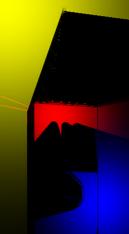
The left image is the input scene, where dark pixels are solid obstacles. The right image shows the result of lighting the scene with three lights of different colors in different positions. The light “passes through” lighter-colored pixels and stops at the obstacles.
Images
A raster image is a 2D array of pixels, each of which has a color. An extremely common way to represent colors is with three 8-bit integers for the red, green, and blue components.
See the image.h file for definitions of the Color and Image structs that reflect this strategy.
The Image struct is a wrapper around a row-major array of Colors.
We have also provided utilities to read and write images in the ubiquitous PNG format.
Illumination
Your work on this assignment will add lighting effects to raster images. The main task is to compute the illumination for every pixel in the image: how much the pixel is lit by the light sources in the scene.
For an unobstructed pixel (i.e., there is not a solid object between the pixel and the light source), here is a formula for the illumination of that pixel by that one light:
\[ \text{illumination} = (\text{light color}) \times e^{\frac{-(\text{distance to light})^2 }{ \text{light strength}}} \]
This formula makes illumination decay with distance.
The color and strength are intrinsic properties of the light source.
(The raycaster_util.h header defines a Light struct with these fields.)
Multiplying a color by a number scales its intensity by multiplying the red, green, and blue components by the same amount.
We have provided an implementation of this function as the illuminate function in raycaster_util.c.
Remember that this illumination formula is only relevant when there is no occlusion (no obstacle between the light and the given pixel).
A single pixel may be illuminated by multiple light sources.
Use the add_colors function from image.h to combine the illumination from multiple lights.
The Input Scene
In general, there are many ways to specify the scene data for a renderer. In our setup, the scene comes as an image, where light pixels represent free space and dark pixels are solid obstacles. Specifically, a pixel is a solid obstacle if:
\[ \text{red} + \text{green} + \text{blue} \lt 10 \]
We have provided an implementation of this formula as is_obstacle in raycaster_util.h.
Casting Rays
The core of the algorithm is the occlusion check: for a given destination pixel and a given light, check every pixel on a line segment between the destination and the light for a solid obstacle.
The idea is to iteratively move along this line segment by some distance, one step at a time:
\[ \text{next pixel} = \text{current pixel} + \text{direction} \times \text{distance} \]
Due to an interesting physics result called Helmholtz reciprocity, both of the following approaches are, in theory, mathematically equivalent:
- start at a light and move toward a pixel in the image
- start at a pixel in the image and move toward a light
However, we recommend that you go with the light-to-pixel approach since there can be slight differences in practice, and our autograder is made with this approach in mind.
This strategy requires the direction (i.e., angle) from each light source to each destination pixel. Let the destination pixel be \((x, y)\) and let the light be at \((i, j)\). Recalling our trigonometry classes, we can calculate the direction as:
\[ \text{direction} = \text{atan}\left(\frac{y - j}{x - i}\right) \]
We have provided an implementation of this formula as direction_pair in raycaster_util.h.
This step-by-step strategy also requires a distance.
We want to step in the calculated direction just far enough to reach the next pixel.
We have implemented the distance calculation in a function called step (also in raycaster_util.h), which moves from an input pixel in a given direction to a neighboring pixel.
To trace a ray, iteratively call step to test every pixel on the line segment between the light and the destination pixel.
The light-source pixel itself is always illuminated.
Pixels containing solid objects are never illuminated.
Task 1: Sequential Raycast Implementation
Your first task is to implement the 2D raycasting algorithm described above.
Implement the raycast_sequential function in raycaster.c:
Image* raycast_sequential(Image* scene, Light* lights, int light_count);
This function takes in an input image that describes the scene and an array of light sources. It produces a rendered image of the same size.
For every pixel \((i, j)\) in the image, compute the illumination of that pixel for every light. Remember to handle occlusion, i.e., do not include contributions from lights that have a solid obstacle “in the way.”
Let the original color of a given pixel in image be called orig.
Call the combined illumination color, across all lights, illum.
The final output color of that pixel in image should be mul_colors(illum, orig).
(The mul_colors function in image.h performs a normalized multiplication in each of the red, green, and blue channels.)
The result is an image that looks like the original but colors the “empty space” according to the illumination at that point.
Some Useful Functions
Please look through raycaster_util.h and image.h for many functions you can use to implement your algorithm.
Here are some particularly important ones, most of which we have already alluded to above:
Color illuminate(Light light, int x, int y)calculates our equation for illumination for a single point at a single non-occluded point.int is_obstacle(Color color)decides whether a given pixel is a solid obstacle.int adjacent_pixels(PixelLocation pixel1, PixelLocation pixel2)determines whether two given pixels are adjacent to each other.Pair direction_pair(PixelLocation start, PixelLocation end)finds the direction (angle) between two points.PixelLocation step(Pair* pos, Pair direction)moves a pixel position by one pixel in the given direction, which is useful for tracing the line segment representing each light ray. The in/out parameterposis a floating-point position that can represent fractional coordinates; it is mutated to reflect the new location. See the documentation comment inraycaster_util.hfor more details.Color add_colors(Color color1, Color color2)adds two color values together, for combining the effects of multiple lights.Color mul_colors(Color color1, Color color2)multiplies two colors, for applying the illumination color to the original pixel.Image* new_image(int width, int height)allocates a new, empty image. Use this to create the output image for all your raycaster implementations.Color* image_pixel(Image* image, int x, int y)gets a pointer to one pixel in an image at the given coordinates. This is just a one-liner that does the row-major index math (which some might prefer to write themselves).
Running and Testing
For a quick-and-dirty smoke test, use main.c.
This program uses a hard-coded input image and light arrangement;
you should experiment with different images and lights by manually modifying main.c.
Use rv make raycaster to produce the raycaster executable.
Running this executable (via rv qemu ./raycaster) produces raycast.png, which you can open in any image viewer.
We have also provided a more systematic testing framework in test_raycaster.c.
Use rv make test_raycaster to build a test_raycaster executable. Use rv qemu ./test_raycaster to run the test executable.
This tool uses inputs from your images/ directory and compares the results against reference outputs in images/test_references/.
It also saves the actual output images from your raycaster in images/sequential_results/ so you can inspect them visually if you like.
Expand the Test Suite
You must add at least 5 new tests to the test suite in test_raycaster.c.
For the sequential implementation, this means adding new input image files (scenes) and corresponding lines in test_raycast_sequential, possibly with different light positions.
Here are some ideas for kinds of tests you might add:
- Very small images that act as “unit tests” for specific edge cases.
- Different light positions for the existing images in the
images/directory. - New input scenes that you draw yourself using an image editor.
Make sure your implementation passes the given tests and your own new tests. It is important to be confident that your sequential implementation is correct before moving on to the parallel versions.
If you add new image files to go with your tests, you can optionally turn these in alongside your test code.
Task 2: Light-Parallel Raycast Implementation
In this and the next task, you will implement parallel versions of the raycaster. The first strategy uses parallelism over the light sources. The insight is that it is possible to independently compute the illumination due to each light. So we can use multiple threads to process subsets of the lights. The threads will then need to somehow coordinate to combine the contributions from separate lights and to produce the final image.
Complete this function in raycaster.c:
Image* raycast_parallel_lights(Image* scene, Light* lights, int light_count, int max_threads);
Your implementation may use up to max_threads parallel threads.
If there are fewer lights than max_threads, then you can use light_count threads (with one light per thread).
If there are more lights than max_threads, then each thread will have to process more than one light.
Use the pthreads library for all your thread creation, management, and synchronization needs.
Some useful functions include: pthread_create, pthread_join, pthread_mutex_lock' and 'pthread_mutex_unlock. Refer to lab 13 for background on how to use these functions and threads in general.
The exact strategy for how to distribute work among threads and when to synchronize is up to you.
But be sure to unsynchronize accesses to shared data:
if two different threads might write the same variable, for example, use some pthreads synchronization construct to enforce exclusive access.
This parallel function, as well as the following one in Task 3, can be correctly implemented either with or without a mutex. Consider how the order of logic in these two functions may differ based on your implementation choice.
Test your implementation with test_raycaster.c.
Your parallel implementation should produce the same results as your sequential implementation.
Task 3: Column-Parallel Raycast Implementation
Next, we will use a different strategy to parallelize the same work. The idea is to parallelize the computation for different parts of the image. Namely, we will divide the columns (\(x\)-coordinates) of pixels among threads.
Implement this function in raycaster.c:
Image* raycast_parallel_columns(Image* scene, Light* lights, int light_count, int max_threads);
Again, the max_threads parameter describes how many threads your implementation can use.
You must divide the image’s columns among max_threads threads (unless the width is less than max_threads, in which case you will have one thread per column).
And once again, test your work using test_raycaster.c to ensure that your new implementation matches your sequential implementation.
Collecting Timing Data
If you would like to test your performance, it would be a good use of your time to partially or completely automate the data collection process. Collecting this data isn’t required, but it may help reveal mistakes in your implementation or reveal how your code scales with different parameters (image size, number of lights/threads, etc.).
To help you get started, we have provided a basic data-collection program timing.c that you can adapt to your needs.
Modify this as much as you like; you will not turn it in.
You can start by changing the constants at the top of the file:
FILENAME(the input image),LIGHT_NUMBER(the program generates lights in a grid pattern),ITERATIONS(how many times to repeat the raycasting execution to measure an average execution time), andTHREAD_COUNT.
The current program only measures one parameter configuration at a time; you might consider extending it to try multiple configurations in a single run.
Use rv make timing to build the timing executable from timing.c.
Submission
On Gradescope, submit raycaster.c and test_raycaster.c (with your 5 additional tests).
Rubric
- Implementation: 60 points
raycast_sequential: 20raycast_parallel_lights: 20raycast_parallel_columns: 20
- Additional Tests: 10 points