Chapter 3 Analyzing Best-Response Dynamics

In this chapter, we present the first simple connection between game theory and graph theory: we use graphs to analyze games and best-response dynamics. Using this graph-theoretic approach, we will be able to give a simple characterization of the class of games for which best-response dynamics converge. The characterization, as well as the method used to prove it, will be useful in the sequel.

3.1 A Graph Representation of Games

We can use graphs to analyze (normal-form) games as follows. Given a game $𝒢 = (n, A, \vec{u})$ , consider a directed graph $G$ where the set of vertices is the set $A$ of action profiles, and where we put a (directed) edge from a node $\vec{a}$ to a node ${\vec{a}}^{'}$ if and only if there exists some player $i$ such that (1) $\vec{a}$ and ${\vec{a}}^{'}$ differ only in component $i$ (i.e., $i$ ’s action) and (2) $a_{i} \notin B R_{i} (\vec{a})$ but $a_{i}^{'} \in B R_{i} (\vec{a})$ ; that is, draw an edge between action profiles if we can go from the first action profile to the second in one step of BRD (i.e., one player improving its utility by switching to its best response). See Figures 3.1 and 3.2 for examples of such graphs for Bach–Stravinsky and the Traveler’s Dilemma.

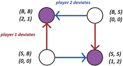
**Figure 3.1:** A BRD graph for the Bach–Stravinsky game. Sinks (i.e., equilibria) are marked in purple. Observe that there are multiple sinks reachable from each non-equilibrium outcome, depending on which player deviates.

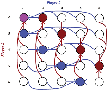
**Figure 3.2:** A small part of the BRD graph for Traveler’s Dilemma, illustrating why this game converges to the equilibrium of (2, 2). Nodes that can be reached as a best response by player 1 are marked in red, and those than can be reached as a best response by player 2 are marked in blue; the sink is marked in purple.

We can now reinterpret BRD and PNE using standard graph-theoretic notions:

The BRD process can be interpreted as simply starting at any node $\vec{a}$ in $G$ and then picking any outgoing edge, traversing it to reach a new node ${\vec{a}}^{'}$ , picking any outgoing edge from it and so on. That is, we take a walk from any node in the graph.

BRD converges in

𝒢

if and only if there are no cycles in

G

—that is,

G

is a acyclic. This means that we eventually reach a node that does not have any outgoing edges and thus the path ends.

By Claim 1.4,

\vec{a}

is a PNE if and only if

\vec{a}

is a sink (i.e., a node without any outgoing edges) in the graph

G

. If a node is a sink in

G

, no one can improve their utility by best responding, and thus

\vec{a} \in B R (\vec{a})

Note that it is not necessary that all nodes reach the same sink for BRD to converge; as in the Bach–Stravinsky game, some games can have multiple equilibria, or even multiple equilibria reachable from the same starting profile.

3.2 Characterizing Convergence of BRD

We can now use this graph representation to characterize the set of finite games for which BRD converges. Given a game $𝒢 = (n, A, \vec{u})$ , we define a potential (or “energy”) function $Φ : A \to ℤ$ , which maps outcome profiles to integers (denoting the “energy level”). A particularly natural potential function (which we will use later) is the utilitarian social welfare, or simply social welfare (SW), defined as the sum of all players’ utilities:

Φ (\vec{a}) = SW (\vec{a}) = \sum_{i \in [n]} u_{i} (\vec{a}) .

The notion of an ordinal potential function will be useful. Roughly speaking, a potential function is said to be ordinal if any profitable single-player deviation increases the potential:

Definition 3.1. $Φ : A \to ℤ$ is an ordinal potential function for a game $𝒢 = (n, A, \vec{u})$ if, for every action profile $\vec{a} \in A$ , every player $i$ , and every action $a_{i}^{'} \in A_{i}$ , if

u_{i} (a_{i}^{'}, a_{- i}) > u_{i} (a_{i}, a_{- i})

then

Φ (a_{i}^{'}, a_{- i}) > Φ (a_{i}, a_{- i}) .

We may also consider a weaker form of a potential function, which we refer to as weakly ordinal, which simply requires the potential to increase for any profitable single-player deviation to a best response.

Definition 3.2. $Φ : A \to ℤ$ is a weakly ordinal potential function for a game $𝒢 = (n, A, \vec{u})$ if, for every action profile $\vec{a} \in A$ , every player $i$ , and every action $a_{i}^{'} \in A_{i}$ such that $a_{i} \notin B R_{i} (\vec{a})$ but $a_{i}^{'} \in B R_{i} (\vec{a})$ , we have that

Φ (a_{i}^{'}, a_{- i}) > Φ (a_{i}, a_{- i}) .

Note that if $Φ$ is ordinal, then it is clearly also weakly ordinal, since if $a_{i} \notin B R_{i} (\vec{a})$ but $a_{i}^{'} \in B R_{i} (\vec{a})$ then $u_{i} (a_{i}^{'}, a_{- i}) > u_{i} (a_{i}, a_{- i})$ .

We now have the following characterization of the class of finite games for which BRD converges.

Theorem 3.1. BRD converges in a finite game $𝒢$ if and only if $𝒢$ has a weakly ordinal potential function.

Proof. We will prove each direction separately.

Claim 3.1. If a finite game $𝒢$ has a weakly ordinal potential function, then BRD converges in $𝒢$ .

Proof. Consider an arbitrary starting action profile (node) $\vec{a}$ , and consider running BRD starting from $\vec{a}$ . Each time some player best responds, the potential $Φ$ increases. Since the game has a finite number of outcomes, there are only a finite number of possible potentials; thus, after a finite number of best response steps, we must have reached the highest possible potential, which guarantees convergence as no more “deviations” are possible from that point.

■

Claim 3.2. If BRD converges in a finite game $𝒢$ , then $𝒢$ has a weakly ordinal potential function.

Proof. Consider some game $𝒢$ where BRD converges, and consider the induced graph representation $G$ of $𝒢$ . As noted above, since BRD always converges, $G$ is a acyclic, and thus every path from any starting point $\vec{a}$ must eventually lead to a sink. We construct a potential function $Φ$ for $𝒢$ as follows: for each action profile $\vec{a}$ , let $Φ (\vec{a}) = - ℓ (\vec{a})$ where $ℓ (\vec{a})$ is the length of the longest path from $\vec{a}$ to any sink $s$ in $G$ . (In other words, $l (\vec{a})$ is the largest number of steps that BRD can take to converge, starting from $\vec{a}$ .)

We now show that each time we traverse an edge in the BRD graph $G$ (i.e., take one step in the BRD process) the potential increases—that is, $ℓ$ decreases. Assume we traversed the edge $(\vec{a}, {\vec{a}}^{'})$ and that $ℓ ({\vec{a}}^{'}) = k$ . Let us then argue that $ℓ (\vec{a}) \geq k + 1$ . This directly follows since there exists some path $p$ of length $k$ from ${\vec{a}}^{'}$ to some sink $s$ , and thus there exists a path of length $k + 1$ from $\vec{a}$ to $s$ by simply first traversing $(\vec{a}, {\vec{a}}^{'})$ and then following $p$ .

■

The theorem directly follows from the above two claims.

■

In the sequel, we will use Theorem 3.1 as a way to show that BRD converges in the games we will be considering. In particular, for all those games, we will exhibit an ordinal potential function (which, as noted above, must also be weakly ordinal), and thus Theorem 3.1 can be used to deduce that BRD converges.

3.3 Better-response Dynamics

The fact that a game has an ordinal (as opposed to just weakly ordinal) potential function is interesting in its own right. In such games, a more general type of best-response dynamics—referred to as better-response dynamics—will always converge: better-response dynamics proceeds exactly as best-response dynamics except that players can switch to any profitable deviation (as opposed to just the best one). More precisely, at every step in the dynamics:

Pick any player $i$ for which $a_{i} \notin B R_{i} (\vec{a})$ , and replace $a_{i}$ by any action in $a^{'} \in A_{i}$ such that
$u_{i} (a_{i}^{'}, a_{- i}) > u_{i} (\vec{a}) .$

In particular, $a_{i}^{'}$ may not necessarily be the optimal response (i.e., a best response) to $a_{- i}$ . For instance, consider the outcome $(70, 50)$ in the Traveler’s Dilemma (which we defined in Section 1.6): player $1$ is currently getting $50 - 2 = 48$ in utility, and could “better-respond” by choosing $50, 49, 48, 47$ ; in contrast, the only best response is choosing $49$ (which would yield utility $51$ ). See Figure 3.3 for an illustration of the (very complicated) “better-response dynamics graph” for the Traveler’s Dilemma.

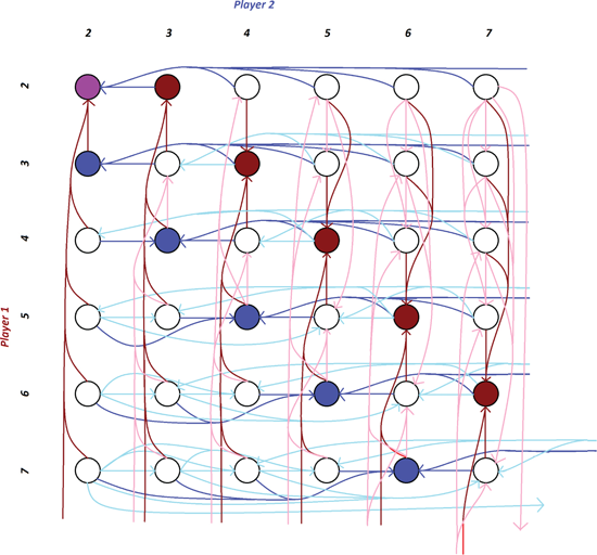
**Figure 3.3:** A small part of the better-response dynamics graph for the Traveler’s Dilemma. The edges that are present in better-response dynamics but not in BRD are indicated in lighter colors. Nodes that can be reached as a best response by player 1 are marked in red, and those than can be reached as a best response by player 2 are marked in blue; the sink is marked in purple.

Better-response dynamics captures situations where it may be hard for players to always find some best response (for instance, if the action space is large) but the players clearly want to change whenever they find some action that improves their utility—i.e., the players simply “myopically” try to improve their utility. Note that, since any valid execution of BRD is also a valid execution of the better-response dynamics, whenever better-response dynamics converges, so does BRD. More generally, we now have the following characterization of the class of games for which better-response dynamics converges.

Theorem 3.2. Better-response dynamics converges in a finite game $𝒢$ if and only if $𝒢$ has an ordinal potential function.

Proof. The proof is essentially identical to the proof of Theorem 3.1, except that in the “only-if direction” we replace the best-response graph by a “better-response graph.”

■

As mentioned, in the sequel, we will use ordinal potential functions to demonstrate convergence of BRD; those proofs thus also show convergence of better-response dynamics.

3.4 Games without PNE

As mentioned in chapter 1, there are finite games—such as the Rock–Paper–Scissors game—without any PNE. For such games, by Claim 1.4, BRD cannot converge. We end this section by illustrating in Figure 3.4 the BRD graph for the Rock–Paper–Scissors game. Notice that there is no sink in this graph; as such, the graph provides a visual proof of the inexistence of PNE in the Rock–Paper–Scissors game.

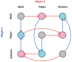
**Figure 3.4:** A BRD graph for a game with no pure strategy Nash equilibrium (Rock–Paper–Scissors).

Notes

The notion of an ordinal potential function and the characterization of games for which better-response dynamics converge is due to Monderer and Shapley [MS96]. The use of potential functions to prove the existence of PNE dates back to the work by Rosenthal [Ros73].