Chapter 2 Graphs

Graphs—sets of nodes connected by edges—are extremely important mathematical objects that arise quite often in real-life applications. For instance:

In a computer network, we can model how all the computers are connected to each other as a graph. The nodes correspond to computers, and edges exist between computers that are connected to each other. This graph is obviously important for routing messages between the computers (e.g., to answer questions such as “What is the fastest route between two computers?”).
Consider a graph representing a map, where the edges correspond to roads and the nodes correspond to points of intersection and cities. How can we find the shortest path from point A to point B? (Some roads may be one way, and we thus need the concept of directed edges to capture this.)
We can model the Internet as a graph: nodes correspond to webpages, and directed edges exist between nodes for which there exists a link from one webpage to the other. As we shall discuss in more detail in chapter 15, this structure is very important for Internet search engines: The relevance of a webpage can be determined by how many links are pointing to it (and recursively how important those webpages are).
Social networks can be modeled as graphs: nodes correspond to people, and we draw (undirected) edges between nodes (i.e., people) who are friends with each other.

In this chapter, we will discuss some basic properties of graphs, and present some simple algorithms for exploring them. (We return to some more advanced algorithms in chapter 6.)

2.1 Basic Definitions

Let us start by defining the notions of directed and undirected graphs. See Figure 2.1 for an illustration.

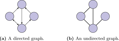
**Figure 2.1:** A basic example of directed and undirected graphs.

Definition 2.1. A directed graph, or simply graph, $G$ , is a pair $(V, E)$ where $V$ is a set of vertices (or nodes), and $E \subseteq V \times V$ is a set of edges. We say that $G$ is an undirected graph if for every pair of nodes $u, v \in V$ , $(u, v) \in E$ if and only if $(v, u) \in E$ (i.e., all edges are “bidirectional”).

Given an undirected graph $G = (V, E)$ , to simplify notation, we often represent the pair of edges $(u, v), (v, u) \in E$ as a single unordered pair ${u, v}$ ; that is, for undirected graphs $G = (V, E)$ , $E \subseteq {{u, v} | u, v \in V}$ . Given an edge $e = (u, v)$ in a graph $G$ , we say that $e$ is outgoing from $u$ and incoming to $v$ . Note that it can be the case that $u = v$ in which case we refer to the edge $e = (u, u)$ as a self-loop. When we refer to the size of a graph $G = (V, E)$ (denoted $| G |$ ), we mean the number of vertices $| V |$ in the graph; that is, $| G |$ is defined as $| V |$ . A complete graph $G = (V, E)$ is a graph where $E = V \times V$ ; that is, we have an edge between any two nodes $u, v \in V$ .

A subgraph of a graph $G = (V, E)$ is a smaller graph on a subset of nodes from $V$ consistent with the edges from $E$ . More formally,

Definition 2.2. Given a graph $G = (V, E)$ , a subgraph of $G$ is a graph $G^{'} = (V^{'}, E^{'})$ where $V^{'} \subseteq V$ and $E^{'} \subseteq (V^{'} \times V^{'}) \cap E$ . We use the notation $G^{'} \subseteq G$ to denote that $G^{'}$ is a subgraph of $G$ .

We turn to defining the notion of node degree:

Definition 2.3. In a graph $G = (V, E)$ , the in-degree of a node $v \in V$ , denoted $in-deg (v)$ , is the number of edges incoming to $v$ (i.e., edges $e \in E$ of the form $e = (u, v)$ ); the out-degree of $v$ , denoted $out-deg (v)$ , is the number of edges outgoing from $v$ (i.e., edges $e \in E$ of the form $e = (v, u)$ ). The degree of $v$ , denoted $deg (v)$ , is the sum of the in-degree and the out-degree of $v$ .

We refer to a node that has in-degree $0$ (i.e., no incoming edges) as a source, and a node with out-degree $0$ (i.e., no outgoing edges) as a sink. Pictorially, the degree of a vertex corresponds to the number of “lines” going in or out from the vertex. (Note that self-loops contribute twice to the degree of a vertex.)

2.2 Connectivity and Reachability

We turn to consider the notion of connectivity. We first define what it means for a node $v^{'}$ to be reachable from (or connected to) a node $v$ .

Definition 2.4. A path (or walk) in a graph $G = (V, E)$ is a sequence of vertices $(v_{1}, v_{2}, \dots, v_{k})$ such that there exists an edge between any two consecutive vertices (i.e., $(v_{i}, v_{i + 1}) \in E$ for $1 \leq i < k$ ). We refer to $k$ as the length of the path. If $k > 1$ and $v_{1} = v_{k}$ (i.e., the starting vertex is the same as the ending vertex), we refer to the path as a cycle. We say that a node $v^{'}$ is reachable from $v$ (or connected to $v$ ) if there exists a path from $v$ to $v^{'}$ .

A graph without cycles is called acyclic. We turn to defining what it means for a graph to be connected. For simplicity, we will restrict our attention to undirected graphs.

Definition 2.5. An undirected graph $G = (V, E)$ is connected if there exists a path between any two nodes $u, v \in V$ . (Note that a graph containing a single node $v$ is considered connected via the length 0 path $(v)$ .) If an undirected graph is not connected, we say that it is disconnected.

When an undirected graph is disconnected, we may decompose the graph into smaller connected components.

Definition 2.6. A connected component of an undirected graph $G = (V, E)$ is a maximal connected subgraph—that is, a subgraph $H \subseteq G$ that is connected, and any larger subgraph $H^{'}$ (satisfying $H^{'} \neq H$ , $H \subseteq H^{'} \subseteq G$ ) must be disconnected.

See Figure 2.2 for an illustration of connected components of a graph.

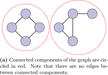
**Figure 2.2:** Example of connected components.

Let us note an intersting application of connectivity to social networks. It has been experimentally observed that in social networks (e.g., Facebook), although not everyone is in the same connected component, most people typically are: we informally refer to this component as the giant component. One reason for why most people are part of the same giant component is that if we had two (or more) large components in the graph, then all it takes to “merge” two large components into a single larger component is for one of the people in each component to become friends—it is very unlikely that this does not happen for any such pair of people. (This argument can be formalized in Erdős and Renyi’s “random graph” model [ER59, Bol84]; we discuss the random graph model in more detail below.)

2.3 Breadth-first Search and Shortest Paths

How do we check if there is a path from $v$ to $v^{'}$ ? One efficient way to do this is with breadth-first search (BFS). Breadth first search is a basic graph search algorithm that given a graph $G$ and a starting node $v$ proceeds as follows: visit all the neighbors $v^{'}$ of $v$ , then visit all the currently unvisited neighbors of those nodes $v^{'}$ , and so on and so forth, while keeping track of which nodes have previously been visited. More precisely,

Step 0: Mark $v$ as visited.
Step 1: Traverse the edge between $v$ and every currently unvisited neighbor $v^{'}$ of $v$ . Mark all those neighbors $v^{'}$ as visited (and for each such neighbor $v^{'}$ , store a “back-pointer” to $v$ ).
Step $k > 1$ : For every node $v^{'}$ marked as visited in step $k - 1$ , traverse any edge between $v^{'}$ and some currently unvisited neighbor $v^{″}$ of $v^{'}$ ; mark all those neighbors $v^{″}$ as visited (and for each such neighbor $v^{″}$ , store a “back-pointer” to $v^{'}$ ).

See Figure 2.3 for an illustration of the execution of the BFS algorithm.

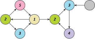
**Figure 2.3:** An illustration of breadth-first search. Starting from node $S$ , in the first step we visit all of the neighbors of $S$ (marked with a 1), in the second step we visit all of the unvisited neighbors (marked with a 2) of each node visited in the first step, and so on. Notice that, in four steps, BFS visits every node except for the top-right node (unlabeled), which clearly has no path from $S$ .

As we now show, the BFS algorithm can be used not only to determine whether there exists a path from $v$ to $v^{'}$ , but also to find some shortest path (i.e., a path of minimal length) between $v$ and $v^{'}$ .

Claim 2.1. For all vertices $v, v^{'}$ , if there exists a path from $v$ to $v^{'}$ , the BFS algorithm starting from vertex $v$ traverses some shortest path from $v$ to $v^{'}$ (and this shortest path can be retrieved by following the “back-pointers” from $v^{'}$ ).

Proof. Assume for contradiction that there exists a path from $v$ to $v^{'}$ , but that the BFS algorithm does not traverse any shortest path from $v$ to $v^{'}$ . Let $(v_{0} = v, v_{1}, v_{2}, \dots, v_{n} = v^{'})$ be a shortest path from $v$ to $v^{'}$ , and let $v_{i}$ be the first node on the path such that BFS does not traverse a path of length (at most) $i$ from $v$ to $v_{i}$ . Such a node must exist because, by assumption, BFS does not traverse a path of length $n$ from $v = v_{0}$ and $v^{'} = v_{n}$ ; additionally $i \geq 1$ , since $v_{0} = v$ is the starting point.

Since $v_{i}$ is the first node on the path for which BFS fails to traverse a path of length at most $i$ , it must have traversed a path of length at most $i - 1$ to get to $v_{i - 1}$ . Consequently, after visiting $v_{i - 1}$ , BFS will visit $v_{i}$ since it is a neighbor of $v_{i - 1}$ that still is unvisited at this point (or else BFS would have traversed a path of length at most $i - 1$ to get from $v$ to $v_{i}$ ). Thus, BFS traverses a path of length at most $i$ from $v$ to $v_{i}$ , which is a contradiction.

■

As a consequence of the above claim, and observing that BFS will only visit each node once (and thus its running time is polynomial in the number of nodes in the graphs), we have the following theorem.

Theorem 2.1. Shortest paths in a graph $G$ can be found in polynomial time in $| G |$ .

Since running BFS from a node $v$ visits all the nodes that are reachable from $v$ (by Claim 2.1), we also have the following result.

Theorem 2.2. Given any node $v$ in $G$ , the set of nodes that are reachable from $v$ in $G$ can be found in polynomial time in $| G |$ .

We can also use BFS to find the connected components of an undirected graph $G$ : Start at any node $v$ and use BFS to find the set of nodes that are reachable from $v$ ; by the definition of reachability, the subgraph corresponding to those nodes is the maximal connected subgraph containing $v$ and thus a connected component. Mark all those nodes as component 1. Next, take some currently unmarked node $v^{'}$ , and again use BFS to find the set of nodes that are reachable from $v^{'}$ ; mark all those notes as component 2. Continue in the same manner until all nodes have been marked.

Some applications of BFS and shortest paths to social networks include the following:

The “Bacon number” of an actor or actress is the length of the shortest path from an individual to the actor Kevin Bacon in the undirected graph where the nodes are actors and actresses, and edges connect people who star together in a movie. The “Erdős number” is similarly defined to be the distance of an individual to the mathematician Paul Erdős in the co-authorship graph.

Milgram’s small-world experiment [Mil67] (a.k.a. the six degrees of separation) demonstrates that everyone is approximately six steps away from anyone else in a social network: random people in Omaha were asked to forward a letter to a “Mr. Jacobs” in Boston, but they could only forward the letter through someone they knew on a first-name basis. Surprisingly, the average path length was roughly 6. This “small-world phenomenon” has since been reconfirmed in multiple subsequent studies. In 1998, Watts and Strogatz [WS98] demonstrated a mathematical model that accounts for this phenomenon.
Milgram’s experiment shows that not only are people connected through short paths, but they also manage to efficiently route messages given only their local knowledge of the graph structure. Jon Kleinberg’s [Kle00] local search model provides a refinement of the Watts–Strogatz small-world model, which can explain how such routing is possible.

To get some intuition for why small-world effects happen, let us consider Erdős and Renyi’s “random graph” model [ER59]:

The random graph model Consider a graph with $n$ nodes, where every pair of nodes has an edge between them (determined independently and with no self-loops) with probability $\frac{1}{2}$ . To gain some intuition about how many nodes have “short paths” between them, we start by asking the following question: What is the probability that two vertices $v$ and $v^{'}$ have a path of length at most 2 between them?

Given any specific third vertex $z$ , the probability of a path $((v, z), (z, v^{'}))$ is only $\frac{1}{2} * \frac{1}{2} = \frac{1}{4}$ . However, since there are $n - 2$ possible “third vertices” for this path, the probability that two nodes are not connected by any path of length exactly 2 is

{(1 - \frac{1}{4})}^{n - 2} = {(\frac{3}{4})}^{n - 2} .

By the Union Bound (see Corollary A.2 in Appendix A), we thus have that the probability that there exists some pair of nodes that is more than distance 2 apart is

\begin{array}{l} Pr [⋃_{u \neq v} u, v has distance > 2] & \leq \sum_{u \neq v} Pr [u, v has distance > 2] \\ \leq \sum_{u \neq v} Pr [u, v has distance \neq 2] \\ = \frac{n (n - 1)}{2} {(\frac{3}{4})}^{n - 2} . \end{array}

This quantity decreases very quickly as the number of vertices, $n$ , increases. Therefore, it is extremely likely that every pair of nodes is at most distance 2 apart.

Needless to say, in a real social network, people are far less likely than probability $\frac{1}{2}$ to be connected, but the number $n$ of nodes is extremely large. Hence, similar arguments apply to show that the average separation between two nodes is relatively small.

Notes

We refer the reader to [CLRS09] and [KT05] for a more in-depth study of graph algorithms, and to [EK10] for connections between graph properties and social networks.