Chapter 4 Coordination in Social Networks

Recall the iPhone/Android game we considered in the introduction. We now have the necessary tools for analyzing it. We begin by considering a simple form of this game on a social network described by an undirected graph.

4.1 Plain Networked Coordination Games

Given some undirected graph $G$ , consider a game $𝒢$ being played by the nodes of the graph (i.e., the nodes represent the players), defined as follows. Each pair of adjacent nodes participate in a two-player “coordination game” (to be defined shortly) and the utility of a node is defined as the sum of the utilities of all games it participated in. Additionally, we require each node to only select a single action (to be used in all the games it participates in).

A bit more precisely, each node in the graph selects a single action (a “product”)—either $X$ or $Y$ —and participates in the following coordination game (where both players get the same utility in every outcome) with each of its neighbors (assume $x, y > 0$ ):

That is,

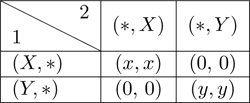
If they “match,” they get the same positive utility $Q (X, X) = x$ or $Q (Y, Y) = y$ ;
If they “mismatch,” they get utility $Q (X, Y) = Q (Y, Y) = 0$ .

Note that the utility, $x$ , of matching on $X$ may be different from the utility, $y$ , of matching on $Y$ . Without loss of generality, we assume $x \geq y$ ; that is, product $X$ is at least as good as product $Y$ . The utility of a node is then defined to be the sum of its utilities in all the coordination games it participates in. Formally,

Definition 4.1. Given an undirected graph $G = (V, E)$ , we say that the game $𝒢 = (n, A, u)$ is a plain networked coordination game induced by $G$ and the coordination utility $Q : {X, Y}^{2} \to ℝ_{\geq 0}$ if:

$V = [n]$ , $Q (X, Y) = Q (Y, X) = 0$ , $Q (X, X) \geq Q (Y, Y) \geq 0$
$A = {X, Y}^{n}$
$u_{i} (\vec{a}) = \sum_{j \in N (i)} Q (a_{i}, a_{j})$ , where $N (i)$ is the set of neighbors of the node $i$ in $G$ .

In the sequel, to simplify notation, we will have some particular plain networked coordination game in mind, and we will let $x$ denote the utility of coordinating at $X$ (i.e., $Q (X, X)$ ) and $y$ the utility of coordinating at $Y$ (i.e., $Q (Y, Y)$ ).

A simple decision rule: The Adoption threshold Consider a node $v$ that has $d$ neighbors (friends), a fraction $p$ of whom choose $X$ and the remaining fraction $(1 - p)$ of whom choose $Y$ . Then $v$ ’s utility for choosing $X$ is $p d x$ and its utility for choosing $Y$ is $(1 - p) d y$ . What action should $v$ take to maximize its utility (i.e., to best respond to the actions of the other players)?

Choose $X$ if $p d x > (1 - p) d y$ —that is, $p > \frac{y}{x + y}$ .
Choose $Y$ if $p d x < (1 - p) d y$ —that is, $p < \frac{y}{x + y}$ .
Choose either $X$ or $Y$ if $p = \frac{y}{x + y}$ .

So, no matter what the number of $v$ ’s neighbors is, the decision ultimately only depends on the fraction of its neighbors choosing $X$ or $Y$ (and the game utilities). We refer to the ratio $t = \frac{y}{x + y}$ as the (global) adoption threshold for product $X$ .

4.2 Convergence of BRD

We now turn to the question of analyzing what equilibria look like in these games. Clearly, everyone choosing the same product is a PNE (everyone choosing $X$ is the “better” equilibrium, but everyone choosing $Y$ is still a PNE). But there are other equilibria as well, such as the ones illustrated in Figure 4.1.

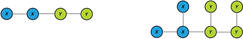
**Figure 4.1:** Illustrations of equilibria in a plain networked coordination game. The left example is an equilibrium when the adoption threshold is $\frac{1}{2}$ or more; the right example shows how to sustain a “nontrivial” equilibrium even when the adoption threshold is smaller, namely, $\frac{1}{3}$ (or more).

Intuitively, the reason why these “nontrivial” equilibria arise is that there is some network structure that “blocks” the better action $X$ from spreading to more nodes in the network. We will return to an analysis of this phenomenon in chapter 5; for now, we will consider the question of whether we can converge to an equilibrium using best-response dynamics.

As we observed in the previous chapter, BRD in a game $𝒢$ converges if and only if $𝒢$ has an ordinal potential function. Here, given a plain coordination game $𝒢 = (n, A, u)$ , we will consider the social welfare function given by

Φ^{𝒢} (\vec{a}) = {SW}^{𝒢} (\vec{a}) = \sum_{i \in n} u_{i} (\vec{a}) .

Whenever the game $𝒢$ is clear from context, we omit it as a superscript for $Φ$ and $S W$ . Notice that by expanding out the definition of $u$ , we get

$Φ^{𝒢} (\vec{a}) = \sum_{(i, j) \in E} Q (a_{i}, a_{j}) = 2 \sum_{{i, j} \in E} Q (a_{i}, a_{j}) .$ (4.1)

Let us now prove that $Φ$ is an ordinal potential function of the game.

Claim 4.1. $Φ^{𝒢}$ is an ordinal potential function for any plain networked coordination game $𝒢$ .

Proof. Consider an action profile $\vec{a}$ and some player $i$ who can improve their utility by deviating to $a_{i}^{'}$ ; that is,

$u_{i} (a_{i}^{'}, a_{- i}) > u_{i} (a_{i}, a_{- i}) .$ (4.2)

We need to show that $Φ (a_{i}^{'}, a_{- i}) > Φ (a_{i}, a_{- i})$ , or equivalently that $Φ (a_{i}^{'}, a_{- i}) - Φ (a_{i}, a_{- i}) > 0$ . Notice that when considering $Φ (a_{i}^{'}, a_{- i}) - Φ (a_{i}, a_{- i})$ , the only games that are affected are those between $i$ and the neighbors of $i$ , $N (i)$ . So, by Equation 4.1, the difference in the potential is

2 \sum_{j \in N (i)} (Q (a_{i}^{'}, a_{j}) - Q (a_{i}, a_{j})) = 2 (u_{i} (a_{i}^{'}, a_{- i}) - u_{i} (a_{i}, a_{- i})),

which by Equation 4.2 is strictly positive.

■

Thus, by Theorem 3.1 (which proved that BRD converges if the game has an ordinal potential function), we directly get the following theorem.

Theorem 4.1. BRD converges in every plain networked coordination game.

Socially optimal outcomes We say that an outcome $\vec{a}$ is socially optimal if it is an outcome that maximizes social welfare; that is, the social welfare in the outcome $\vec{a}$ is at least as high as the social welfare in any other outcome ${\vec{a}}^{'}$ . In other words, $\vec{a}$ is socially optimal in $𝒢$ if

\vec{a} \in arg max_{\vec{a} \in A} S W^{𝒢} (\vec{a}) .

Note that there may not necessarily exist a unique outcome that maximizes social welfare, so several outcomes may be socially optimal.

Let us also remark that if social welfare is an ordinal potential function (as we showed was the case for plain networked coordination games), then whatever outcome we start off with, if people deviate to make themselves better off, they also make the outcome better for “the world in aggregate” (although some players can get worse off). In particular, this implies that if we start out with a socially optimal outcome, BRD will stay there. Note that this is not always the case: for instance in the Prisoner’s Dilemma, the socially optimal outcome is for both players to cooperate, but BRD moves away from this outcomes (as it is not a PNE).

The fact that this happens here, however, should not be too surprising: if $x > y$ , there is a unique outcome that maximizes SW (namely, everyone choosing $X$ ) and this outcome is a PNE, thus BRD will stay there; if $x = y$ , there are two outcomes (everyone choosing $X$ or everyone choosing $Y$ ), which maximize SW, both of which are PNE.

4.3 Incorporating Intrinsic Values

So far we have assumed that players’ utilities depend only on their coordination utilities; in particular, this implies that everyone has the same “intrinsic value” for each product. In reality, people may have different intrinsic value for different products (e.g., in the absence of network effects, some people naturally prefer iPhones and others Androids).

To model this, we can consider a more general class of games where utility is defined as follows:

$u_{i} (\vec{a}) = R_{i} (a_{i}) + \sum_{j \in N (i)} Q (a_{i}, a_{j}) .$ (4.3)

Here, $R_{i} (a_{i})$ denotes the intrinsic value of $a_{i}$ to player $i$ . Formally, the notion of a networked coordination game is defined just as in Definition 4.1, except that we now also parametrize the game by an intrinsic value function $R_{i} : {X, Y} \to ℝ_{\geq 0}$ for each node $i$ and use Equation 4.3 to define utility.

Notice that nodes can no longer employ the same simple decision rule of checking whether the fraction of its neighbors playing $X$ exceeds some fixed global threshold $t$ —rather, each node has its own subjective adoption threshold $t (i)$ that depends on the number of $i$ ’s neighbors and its intrinsic value function $R_{i}$ (Exercise: Derive what the subjective adoption threshold is). Also, notice that it is now no longer clear what equilibria look like, or even that they exist, since there might exist a conflict between the intrinsic value of an action to a player and the desire to coordinate with their friends!

Example 4.1. Consider the simple star graph in Figure 4.2 with $d + 1$ nodes, consisting of a “central” node $v$ connected to $d$ neighbors, and consider the networked coordination game induced by this graph and the following coordination and intrinsic utilities (where $𝜖 > 0$ is some arbitrarily small constant):

Let $R_{v} (X) = d + 𝜖, R_{v} (Y) = 0$ .
For all other nodes $v^{'}$ , $R_{v^{'}} (X) = 0$ and $R_{v^{'}} (Y) = 1 + 𝜖$ .
Let $Q (X, X) = Q (Y, Y) = 1$ (i.e., $x = y = 1$ in the game as described above).

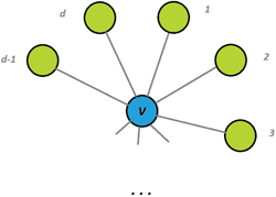
**Figure 4.2:** The star graph described in the example, with the equilibrium outcome highlighted ( $X$ in blue, $Y$ in green).

So every node’s coordination game indicates no network preference between $X$ and $Y$ . But $v$ intrinsically “strongly” prefers $X$ , while all other nodes intrinsically “weakly” prefer $Y$ .

What happens if everyone chooses $X$ in this game?

$v$ has maximized their intrinsic utility ( $d + 𝜖$ ) and maximized coordination utility (1 on each of $d$ edges, for a total of $d$ ), so there is no incentive to switch.

Other nodes currently have no intrinsic utility for

X

and get 1 in coordination utility, so it benefits them to switch to

Y

instead, receiving

1 + 𝜖

in intrinsic utility and losing 1 in coordination utility.

This outcome has social welfare

3 d + 𝜖

, but it is not an equilibrium (since nodes

v^{'} \neq v

gain

𝜖

by switching actions).

What happens if everyone chooses $Y$ ?

Neighbors of $v$ have maximized their intrinsic utility ( $1 + 𝜖$ ) and maximized coordination utility (1), so there is no incentive for them to switch.
$v$ currently has no intrinsic utility and $d$ in coordination utility (1 on each edge), so it benefits $v$ to switch to $X$ instead, receiving $d + 𝜖$ in intrinsic utility and losing $d$ in coordination utility.
This outcome has social welfare $3 d + d 𝜖$ , but it also is not an equilibrium.

In fact, if we apply the BRD process we will always up end in a outcome where $v$ chooses $X$ and the other nodes choose $Y$ , no matter where we start. This follows from the fact that $X$ is strictly dominant for $v$ and $Y$ is strictly dominant for all the other nodes; thus $v$ playing $X$ and everyone else playing $Y$ is the only PNE (and by Claim 1.5, BRD quickly converges to it).

But in this outcome, there is no “coordination” utility; $v$ receives $d + 𝜖$ in intrinsic utility and the other nodes receive $1 + 𝜖$ each, for a total of only $2 d + (d + 1) 𝜖$ in social welfare. There is actually quite a significant gap—a factor of close to $\frac{3}{2}$ —between the equilibrium and the “coordination” outcomes where everyone plays either $X$ or $Y$ . In fact, it is not hard to see that the outcome where everyone plays $Y$ is the only socially optimal outcome in this game; we leave it as an exercise to prove this. We refer to the existence of such a gap as an inefficiency of equilibria (i.e., that selfish behavior leads to “inefficient” outcomes).

Furthermore, notice that this gap is essentially independent of the number of nodes, $d + 1$ , as long as $d \geq 1$ . Thus, an even simpler example illustrating this gap is obtained by simply considering the case when $d = 1$ —that is, we are simply playing a coordination game between two players. (We consider the slightly more complicated star example as it illustrates the issue even in a connected graph with a large number of nodes.)

Can we still prove that equilibria always exist networked coordination games (with intrinsic values) by showing that best-response dynamics converge? Social welfare is no longer an ordinal potential function; as a counterexample, consider the outcome in the graph above where all nodes choose $Y$ . If $v$ switches to $X$ , improving their own utility, the social welfare actually decreases by $d - 𝜖$ (from $3 d + d 𝜖$ to $2 d + (d + 1) 𝜖$ ), even though $v$ actually only increases their utility by $𝜖$ (which can be arbitrarily small)!

However, we can choose a better potential function that is ordinal; namely:

Φ^{'} (\vec{a}) = \sum_{{i, j} \in E} Q (a_{i}, a_{j}) + \sum_{i \in V} R_{i} (a_{i}) .

That is, we sum coordination utilities over every edge once (rather than twice as in the definition of social welfare; see Equation 4.1), and add the intrinsic values for each node.

Theorem 4.2. BRD converges in every networked coordination game.

Proof. Let $Φ^{'}$ be above-described potential function; by Theorem 3.1, it suffices to show that it is ordinal. Consider an action profile $\vec{a}$ and some player $i$ who can improve their utility by deviating to $a_{i}^{'}$ ; that is,

u_{i} (a_{i}^{'}, a_{- i}) > u_{i} (a_{i}, a_{- i}) .

We will show that $Φ^{'} (a_{i}^{'}, a_{- i}) - Φ^{'} (a_{i}, a_{- i}) > 0$ . Once again, in considering $Φ^{'} (a_{i}^{'}, a_{- i}) - Φ^{'} (a_{i}, a_{- i})$ , note that only coordination games between $i$ and $N (i)$ and the intrinsic value for $i$ are affected by changing $a_{i}$ to $a_{i}^{'}$ . So,

$\begin{array}{rcl} Φ^{'} (a_{i}^{'}, a_{- i}) - Φ^{'} (a_{i}, a_{- i}) = \sum_{j \in N (i)} (Q (a_{i}^{'}, a_{j}) - Q (a_{i}, a_{j})) + (R_{i} (a_{i}^{'}) - R_{i} (a_{i})) \\ = u_{i} (a_{i}^{'}, a_{- i}) - u_{i} (a_{i}, a_{- i}) > 0, \end{array}$

which concludes the proof.

■

4.4 The Price of Stability

As we saw in the earlier example, BRD might decrease social welfare—in particular, even a single player best responding once can significantly bring down the social welfare. A natural question thus arising is: How bad can the “gap” between the social welfare in the “best” equilibrium (i.e., the PNE with the largest social welfare) and in the socially optimal outcome be?

More formally, we denote by

M S W^{𝒢} = max_{\vec{a} \in A} S W^{𝒢} (\vec{a})

the maximum social welfare (MSW) obtainable in the game $𝒢$ . In games with non-negative utilities (such as networked coordination games), we refer to the ratio between the MSW and the SW of the best PNE as the price of stability in the game.

Definition 4.2. The price of stability in a game $𝒢$ with non-negative utilities is defined as

\frac{M S W^{𝒢}}{max_{\vec{a} \in P N E^{𝒢}} S W^{𝒢} (\vec{a})},

where $P N E^{𝒢}$ denotes the set of PNE in $𝒢$ .

Roughly speaking, the price of stability measures by how much selfish behavior necessarily degrades the “efficiency” of outcomes. (There is also a related notion of price of anarchy, which is defined as the ratio between MSW and the worst PNE—this notion instead measures by how much selfish behavior can, in the most pessimistic case, degrade performance. In the sequel, however, we will focus only on studying the price of stability.)

As we now show, selfish behavior cannot degrade performance by more than a factor 2.

Theorem 4.3. For every networked coordination game $𝒢$ , there exists a PNE ${\vec{a}}^{'}$ in $𝒢$ such that

S W^{𝒢} ({\vec{a}}^{'}) \geq \frac{1}{2} M S W^{𝒢} .

(In other words, the price of stability in $𝒢$ is at most 2.)

Proof. Observe that for the potential function $Φ^{'}$ defined above, for every $\vec{a} \in A$ ,

S W (\vec{a}) \geq Φ^{'} (\vec{a}) \geq \frac{S W (\vec{a})}{2} .

Now, pick any outcome $\vec{a}$ that maximizes $SW (\vec{a})$ (and thus achieves a SW of MSW). Then run BRD starting from $\vec{a}$ until it converges to some outcome profile ${\vec{a}}^{'}$ —as shown in Theorem 4.2 it will always converge, and this final outcome is a PNE. While SW may decrease at each step, as shown in the proof of Theorem 4.2 $Φ^{'}$ can only increase. Hence, we have

S W ({\vec{a}}^{'}) \geq Φ^{'} ({\vec{a}}^{'}) \geq Φ^{'} (\vec{a}) \geq \frac{S W (\vec{a})}{2} = \frac{M S W}{2}

as desired.

■

Recall that our “star graph” exhibited an example of a game with a gap of close to $\frac{3}{2}$ between the best equilibrium and the socially optimal outcome, whereas Theorem 4.3 shows that the gap can never be more than 2. It turns out that the gap of $2$ is actually tight, but showing this requires a slightly more elaborate analysis appealing to iterated strict dominance.

Theorem 4.4. For every $n \geq 2, 𝜖 > 0$ , there exists some $n$ -player networked coordination game $𝒢$ such that for every PNE ${\vec{a}}^{'}$ in $𝒢$ we have that

S W^{𝒢} ({\vec{a}}^{'}) \leq (\frac{1}{2} + 𝜖) M S W^{𝒢} .

(In other words, the price of stability can be arbitrarily close to 2.)

Proof. Let $G = ([n], E)$ be a complete graph on $n$ nodes. Let $Q (X, X) = 1, Q (Y, Y) = 0$ and for every player $i$ , let $R_{i} (X) = 0, R_{i} (Y) = n - i + 𝜖$ . (See Figure 4.3.) Let $\vec{a} = (X, X, \dots, X)$ ; note that $S W (\vec{a}) = 2 | E | = n (n - 1)$ , and so $M S W \geq n (n - 1)$ . Let us next analyze PNE in this game. We will show that $\vec{b} = (Y, Y, \dots, Y)$ is the only strategy profile that survives iterated strict dominance (ISD); by Claim 1.3 (showing that if a unique strategy survives ISD, it must be the unique NE of the game), it thus follows that $\vec{b}$ is also the only PNE of the game.

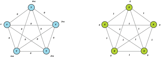
**Figure 4.3:** The construction presented in Theorem 4.4 for $n = 5$ , detailing the intrinsic utilities (next to the nodes) and coordination utilities (on the edges) achieved in (left) the equilibrium and (right) the outcome which maximizes social welfare.

Showing that only $\vec{b}$ survives ISD We will show by induction that after the $k^{th}$ round of ISD, players ${1, \dots, k}$ must have removed action $X$ . The base case ( $k = 0$ ) is trivial. For the induction step, assume the claim is true for round $k$ and let us show it for round $k + 1$ . In the ${(k + 1)}^{th}$ round, by the induction hypothesis, players ${1, \dots, k}$ can only be playing $Y$ . Therefore, player $k + 1$ can get utility at most $n - k - 1$ by playing $X$ (since the intrinsic value of $X$ is 0, and they can can coordinate with at most $n - k - 1$ players); on the other hand, by playing $Y$ , player $k + 1$ is guaranteed to get $n - k - 1 + 𝜖$ (in intrinsic value); thus, $X$ is strictly dominated and must be removed, which proves the induction step.

Concluding the price of stability bound Note that

S W (\vec{b}) = \sum_{i = 1}^{n} R_{i} (Y) = \sum_{i = 1}^{n} (n - i + 𝜖) = \frac{n (n - 1)}{2} + n 𝜖 .

Thus,

\frac{S W (\vec{b})}{M S W} \leq \frac{\frac{n (n - 1)}{2} + n 𝜖}{n (n - 1)} = \frac{1}{2} + \frac{𝜖}{n - 1} .

By choosing an appropriately small $𝜖$ , this value can be made arbitrarily close to 1/2.

■

4.5 Incorporating Strength of Friendship

We finally consider an even more general networked coordination model where we place a “weight” $w_{i, j} = w_{j, i}$ on each (undirected) edge ${i, j}$ —think of this weight as the “strength of the friendship” (measured, for example, by how many minutes we spend on the phone with each other, or how many messages we send to each other)—and now also weigh the coordination utility of the game between $i$ and $j$ by $w_{i, j}$ . That is,

u_{i} (\vec{a}) = R_{i} (a_{i}) + \sum_{j \in N (i)} w_{i, j} Q (a_{i}, a_{j}) .

We note that the potential function, as well as social welfare, arguments made above (i.e., Theorem 4.2 and Theorem 4.3) directly extend to this more general model, by defining

Φ^{'} (\vec{a}) = \sum_{{i, j} \in E} w_{i, j} Q (a_{i}, a_{j}) + \sum_{i \in V} R_{i} (a_{i}) .

Note, however, that a player’s decision whether to play $X$ is no longer just a function of the fraction of their neighbors playing $X$ ; rather, we now need to consider a weighted subjective threshold $t (\cdot)$ where node $i$ switches to $X$ whenever the fraction of their neighbors $j$ weighted by $w (i, j)$ exceeds $t$ .

Notes

The notion of networked coordination games (the way we consider them) was introduced by Young [You02]. Young also showed the existence of PNE in such games.

The gap between the maximum social welfare and the social welfare in equilibria (i.e., the “inefficiency” of equilibria) was first studied by Koutsoupias and Papadimitriou [KP09], but the notion considered there—“price of anarchy”—considered the gap between MSW and the worst PNE. In contrast, the notion of price of stability (which we considered here) considers the gap between MSW and the best PNE. This notion was first studied in [SM03], and the term “price of stability” was first coined in [ADK $^{+}$ 08]; [ADK $^{+}$ 08] was also the first paper to study price of stability using potential functions. The results on price of stability in coordination games that we have presented here are from Morgan and Pass [MP16].

It turns out that the star graph example we presented (and its gap of $\frac{3}{2}$ ) is also tight in some respect: Note that in that example, the coordination game is “coordination symmetric” in the sense that $x = y$ ; for such games, Theorem 4.3 can be strengthened to show that the price of stability never exceeds $\frac{3}{2}$ ; see [MP16] for more details.