Chapter 1 Game Theory

In this chapter, we will develop some basic tools for reasoning about the behavior of strategic agents. The notion of a game is central to this treatment: roughly speaking, a game models a scenario where agents—referred to as players—take some actions and next receive some utility based on their actions; the goal of the players is to maximize their own utility. To gain some intuition for this treatment, we begin by discussing one of the most basic and well-known games in the field: the Prisoner’s Dilemma.

1.1 The Prisoner’s Dilemma Game

Two robbers were caught after robbing a bank. They are put into separate rooms and given the choice to either defect (D)—accuse their partner, or cooperate (C)—stay silent.

If both robbers defect (i.e., accuse their partner), they are both charged as guilty and sentenced to 4 years in prison.
If both cooperate (i.e., remain silent), there is less evidence to charge them and they will both get 1 year in prison.
However, if one robber cooperates (remains silent) and the other defects (accuses their partner), the cooperating one gets 10 years in prison, while the defecting one goes free.

How should the robbers act?

To study this situation, we can represent it as a game: we have two players (the robbers)—let us call them player 1 and 2—and each player needs to choose one of the two actions, $C$ or $D$ . To analyze how these players should act we also need to translate the “desirability” of each possible outcome of the game into a “score” for each player, referred to as the utility of the outcome (where more desirable outcomes are assigned a higher score). This is done by defining utility functions $u_{1}, u_{2}$ for each of the players, where $u_{i} (a_{1}, a_{2})$ denotes the utility (i.e., “score”) of player $i$ in the outcome where player 1 chose the action $a_{1}$ and player 2 chose $a_{2}$ . For instance, let:

$u_{1} (D, D) = u_{2} (D, D) = - 4$ (since both players get 4 years of jail)
$u_{1} (C, D) = - 10$ , $u_{2} (C, D) = 0$ (since player 1 gets 10 years of prison and player 2 goes free)
$u_{1} (D, C) = 0$ , $u_{2} (D, C) = - 10$ (since player 2 gets 10 years of prison and player 1 goes free)
$u_{1} (C, C) = u_{2} (C, C) = - 1$ (since they each get 1 year in prison)

We can represent this game as a table, as follows:

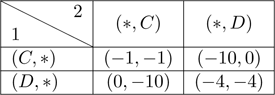
Notice that each player gets strictly more utility by defecting rather than cooperating, no matter what the other player does: $u_{1} (D, *) > u_{1} (C, *)$ and $u_{2} (*, D) > u_{2} (*, C)$ regardless of what action $*$ is. Thus, if both robbers are “rational” and want to maximize their own utility, one would expect both of them to defect in this game, which results in both ending up in prison for 10 years (despite the fact that they could both have been free after 1 year, if they had just both cooperated)!

We turn to formalizing the notion of a game, and subsequently this way of reasoning.

1.2 Normal-form Games

We will focus on a restricted class of games, satisfying the following properties:

Players act only once;
Players act simultaneously (i.e., without knowledge of what the other player will do);
The number of players is finite.

Despite its simplicity, this class of games will suffice for most of the applications we will be considering here. The formal definition follows.

Definition 1.1. A normal-form game is a tuple $𝒢 = (n, A, \vec{u})$ , where

$n \in ℕ$ (the number of players);
$A = A_{1} \times A_{2} \times \dots \times A_{n}$ is a product of sets; we refer to $A_{i}$ as the action space of player $i$ , and refer to the product space, $A$ , as the outcome space;
$\vec{u} = (u_{1}, \dots, u_{n})$ is a vector of functions such that $u_{i} : A \to ℝ$ (that is, $u_{i}$ is the utility function of player $i$ , mapping outcomes to real numbers).

We will mostly focus on the case where the action spaces for each player is a finite set;¹ we refer to a normal-form game $𝒢$ where $A$ is finite as a finite normal-form game. Additionally, for most of the games that we consider, the actions space is the same for all players (i.e., $A_{1} = A_{2} = \dots = A_{n}$ ).

We refer to a tuple $\vec{a} = (a_{1}, \dots, a_{n}) \in A$ of actions as an action profile, or outcome. As players act only once, the strategy of a player is simply the action they take, and as such we use the terms strategy and action interchangeably; the literature sometime calls such strategies pure strategies. (As we briefly discuss later, one may also consider a more general notion of a strategy—called a mixed strategy—which allows a player to randomize over actions.) We assume that all players know $n$ , $A$ , and the utility functions $\vec{u}$ ; the only thing players are uncertain about is the actions chosen by the other players. Shortly, we shall discuss various ways to reason about how rational agents should act in such a game.

Let us first introduce some more notational details:

Let $[n] = {1, 2, \dots, n}$ ;
Given an action space $A$ , let $A_{- i}$ denote the set of actions for everyone but player $i$ (formally, $A_{- i} = \times_{j \neq i} A_{j}$ );
Similarly, given an action profile $\vec{a}$ , let $a_{- i}$ denote the action profile of everyone but player $i$ ;
We will use $(a_{i}, a_{- i})$ to describe the full action profile where player $i$ plays $a_{i}$ and everyone else $a_{- i}$ ;
To simplify notation, we sometimes directly specify $\vec{u}$ as a function from $A \to ℝ^{n}$ (i.e., a function from outcomes to a vector of utilities where component $i$ specifies the utility of player $i$ ). That is, the $i^{th}$ component of $\vec{u} (\vec{a})$ is $u_{i} (\vec{a})$ .

Formalizing the Prisoner’s Dilemma We can model the Prisoner’s Dilemma game that we discussed above as a finite normal-form game $(n, A, \vec{u})$ , where:

$n = 2$ ;
$A_{1} = A_{2} = \{C, D\}$ ;
u→ is defined as follows:
- – $\vec{u} (C, C) = (- 1, - 1)$ (i.e., $u_{1} (C, C) = u_{2} (C, C) = - 1$ );
- – $\vec{u} (C, D) = (- 10, 0)$ ;
- – $\vec{u} (D, C) = (0, - 10)$ ;
- – $\vec{u} (D, D) = (- 4, - 4)$ .

1.3 Dominant Strategies

In the Prisoner’s Dilemma, we argued that playing $D$ was always the best thing to do. The notion of a dominant strategy formalizes this reasoning.

Definition 1.2. A dominant strategy for a player $i$ in a game $(n, A, \vec{u})$ is an action $a_{i}$ such that, for all $a_{i}^{'} \in A_{i} ∖ {a_{i}}$ and all action profiles $a_{- i} \in A_{- i}$ , we have

u_{i} (a_{i}, a_{- i}) \geq u_{i} (a_{i}^{'}, a_{- i}) .

If this inequality is strict (i.e., $u_{i} (a_{i}, a_{- i}) > u_{i} (a_{i}^{'}, a_{- i})$ ), we call $a_{i}$ a strictly dominant strategy.

The following claim follows from our argument above.

Claim 1.1. Defecting ( $D$ ) is a strictly dominant strategy for both players in the Prisoner’s Dilemma.

The fact that $D$ is strictly dominant is good news in the robber situation we described: the police can put the criminals in prison (assuming they act rationally). But in other situations, the fact that $(D, D)$ is the only “rational outcome” is less of a good thing: We can use the Prisoner’s Dilemma game to model conflicts between countries (in fact, this was one of the original motivations behind the game): Consider two countries deciding whether to disarm (cooperate) or arm (defect), and let the utilities be defined in the same way as in the Prisoner’s Dilemma. If the countries act rationally, we end up in a situation where both arm (although they would have been better off if both disarmed instead). This game can thus be viewed as a simplified explanation of arms races, such as those that took place during the Cold War.

1.4 Iterated Strict Dominance (ISD)

In general, when a game has a strictly dominant strategy, this strategy gives a good indication of how people will actually play the game. But not every game has a strictly dominant, or even just a dominant, strategy. To illustrate this, consider the following game.

The Up-Down game Player 1 can choose to go up ( $U$ ) or down ( $D$ ); player 2 can choose to go left ( $L$ ), middle ( $M$ ), or right ( $R$ ). The following table lists the utilities for each possible outcome:

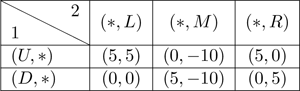
Note that we do not have any strictly dominant actions in this game. So can we say anything about how this game will be played? Note that the action $M$ is always a “terrible” strategy; player 2 would never have any reason to play it. We say that $M$ is strictly dominated by both $L$ and $R$ , by the following definition:

Definition 1.3. Given a game $(n, A, \vec{u})$ , we say that $a_{i} \in A_{i}$ is strictly dominated by $a_{i}^{'}$ (or $a_{i}^{'}$ strictly dominates $a_{i}$ ) for a player $i$ , if for every action profile $a_{- i} \in A_{- i}$ , we have

u_{i} (a_{i}, a_{- i}) < u_{i} (a_{i}^{'}, a_{- i}) .

We say that $a_{i} \in A_{i}$ is (simply) strictly dominated for a player $i$ if there exists some strategy $a_{i}^{'} \in A_{i}$ that strictly dominates $a_{i}$ .

Note that if an action $a_{i}$ is strictly dominant, then it clearly also strictly dominates every other action $a_{i}^{'} \neq a_{i}$ . Also note that strict dominance is transitive—if for player $i$ , strategy $a_{i}$ dominates $b_{i}$ and $b_{i}$ dominates $c_{i}$ , then $a_{i}$ dominates $c_{i}$ . A useful consequence of this is that not all strategies can be strictly dominated (prove it!).

Now, let us return to the Up-Down game. Since $M$ is terrible “no matter what,” we should remove it from consideration. Let us thus consider the resulting game after having removed the action $M$ :

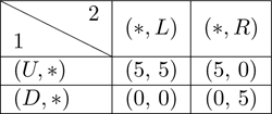
Now look at player 1’s choices; at this point, $D$ is strictly dominated by $U$ and can thus be removed from consideration, resulting in the following game:

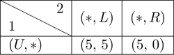
And, finally, player 2 can rule out $R$ , leaving us with $(U, L)$ as the only possible rational outcome. This process is known as iterative removal of strictly dominated strategies, or iterated strict dominance (ISD). In more detail, ISD proceeds in rounds: in each round $j$ , every player $i$ removes all strategies that are strictly dominated with respect to the set of strategies that survived up to set $j - 1$ . In other words, in each round, all players “simultaneously” remove all strictly dominated strategies given the set of strategies that survived in the earlier round. More formally,

Definition 1.4. Given a game $(n, A, \vec{u})$ , we define the set of strategies surviving iterated strict dominance (ISD) as follows:

For each player $i$ , let $A_{i}^{0} = A_{i}$ .
Next, we proceed in rounds: For each round $j \geq 1$ , for each player $i$ , let $A_{i}^{j}$ denote the set of strategies that are not strictly dominated if we restrict the action space to $A^{j - 1} = A_{1}^{j - 1} \times \dots \times A_{n}^{j - 1}$ . That is, $A_{i}^{j}$ is obtained by taking $A_{i}^{j - 1}$ and removing all actions $a_{i}$ for which there exists some $a_{i}^{'} \in A_{i}^{j - 1}$ such that for all $a_{- i} \in A_{- i}^{j - 1}$ , $u_{i} (a_{i}, a_{- i}) < u_{i} (a_{i}^{'}, a_{- i})$ .
Continue this procedure until no more strategies can be removed; that is, $A^{j} = A^{j - 1}$ . Output the final set $A^{j}$ .

Note that since not all strategies can be strictly dominated in a game, this deletion procedure always ends with a non-empty set. Additionally, note that since the deletion procedure is deterministic—we simultaneously remove all dominated strategies in every round—the final set is also unique.

ISD and common knowledge of rationality Intuitively, no “rational” players should ever play a strictly dominated strategy (such as $M$ above)—since it is strictly worse, that would be a silly thing to do. So, if everyone is rational, then nobody will play strictly dominated strategies. Furthermore, if everyone knows that everyone is rational, then, we can effectively restrict our attention to the game where all strictly dominated strategies have been removed (as everybody knows nobody will play them), and then remove dominated strategies from this smaller game. Thus, inductively, if we have common knowledge of rationality—that is, everybody is rational, everybody knows that everybody is rational, everybody knows that everybody knows that everybody is rational, and so forth—people can only play strategies that survive ISD. Later on in the course (in chapter 1.7), we will see how this statement can be formalized: in fact, we show that common knowledge of rationality exactly characterizes the set of strategies that survive ISD, in the sense that a strategy survives ISD if and only if it is compatible with common knowledge of rationality.

1.5 Nash Equilibria and Best-Response Dynamics

Sometimes even iterative strict dominance does not give us enough power to predict the outcome of a game. Consider the following game.

Bach–Stravinsky: A coordination game Two players (husband and wife) are deciding whether to go to a Bach ( $B$ ) or a Stravinsky concert ( $S$ ). The first player prefers Bach and the second Stravinsky, but they will both be unhappy if they do not go together. Formally, $\vec{u} (B, B) = (2, 1)$ , $\vec{u} (S, S) = (1, 2)$ , and $\vec{u} (B, S) = \vec{u} (S, B) = (0, 0)$ . This is a special case of a so-called coordination game where, more generally, the players get “high” utility when they “coordinate” (i.e., choose the same action), and 0 otherwise.

Note that there are no dominant or dominated strategies in this game. So how can we predict what will happen? The classic way to deal with such a situation is to find equilibrium states—namely, action profiles with the property that no individual player can increase their utility by switching strategies, assuming that everyone else sticks to their original strategy. For instance, $(B, B)$ is an equilibrium in this game: if player 1 switched, they would lose 2 in utility, and if player 2 switched, they would lose 1 in utility. Symmetrically, $(S, S)$ is an equilibrium as well.

Pure-Strategy Nash equilibrium (PNE) We now turn to formalizing this notion through what is called a Nash equilibrium.

Definition 1.5. Given a game $(n, A, \vec{u})$ , a pure-strategy Nash equilibrium (PNE) is a profile of action $\vec{a} \in A$ such that for each player $i$ and all actions $a_{i}^{'} \in A_{i}$ ,

u_{i} (\vec{a}) \geq u_{i} (a_{i}^{'}, a_{- i}) .

In other words, there does not exist some player $i$ that has a “profitable deviation”: no player $i$ can increase their own utility by unilaterally deviating, assuming that everyone else sticks to the equilibrium strategy.

Relating PNE and ISD Observe that $(D, D)$ in the Prisoner’s Dilemma and $(U, L)$ in the Up-Down game are both PNEs for their respective games. The following claims show that this was not a coincidence: PNE is a strict refinement of ISD (and thus also strict dominance, since strictly dominant strategies can never be dominated), and when ISD produces a single strategy profile, it must be a PNE.

Claim 1.2. Every PNE survives ISD.

Proof. Consider a PNE $\vec{a}$ , and assume for contradiction that $\vec{a}$ does not survive ISD. Consider the first round $j$ when some player $i$ ’s action $a_{i}$ gets eliminated. Then $a_{- i} \in A_{- i}^{j - 1}$ (since $j$ was the first round when some player’s action in $\vec{a}$ was eliminated). Furthemore, since $a_{i}$ gets eliminated in step $j$ , there must exists some action $a_{i}^{'}$ that strictly dominates $a_{i}$ with respect to $A_{- i}^{j - 1}$ , and hence also with respect to $a_{- i}$ . That is,

u_{i} (a_{i}^{'}, a_{- i}) > u_{i} (a_{i}, a_{- i}) .

But this contradicts the assumption that $\vec{a}$ is a PNE.

■

Claim 1.3. If a single strategy profile survives ISD, then it is the unique PNE of the game.

Proof. Consider some game where a unique strategy profile $\vec{a}$ survives ISD. First, note that by Claim 1.2, there can be at most one PNE in the game (since every PNE survives ISD). Let us next show that $\vec{a}$ must be the (unique) PNE. Assume for contradiction that $\vec{a}$ is not a PNE. That is, there exists a player $i$ and action $a_{i}^{'}$ such that $a_{i}^{'}$ strictly dominates $a_{i}$ with respect to $a_{- i}$ :

$u_{i} (a_{i}^{'}, a_{- i}) > u_{i} (a_{i}, a_{- i}) .$ (1.1)

Since $a_{i}^{'}$ did not survive the deletion process (as only $\vec{a}$ survived ISD by assumption), $a_{i}^{'}$ must have been previously deleted due to being dominated by some strategy $a_{i}^{1}$ , which in turn was deleted by some strategy $a_{i}^{2}$ and so on and so forth, until we reach some strategy $a_{i}^{m}$ that is deleted by $a_{i}$ (since only $a_{i}$ survives ISD). Since $a_{- i}$ was never deleted, we must thus have

u_{i} (a_{i}, a_{- i}) > u_{i} (a_{i}^{m}, a_{- i}) > \dots > u_{i} (a_{i}^{1}, a_{- i}) > u_{i} (a_{i}^{'}, a_{- i}),

which contradicts Equation 1.1.

■

Best responses Another way to think of PNEs is in terms of the notion of a best response. Given an action profile $\vec{a}$ , let $B R_{i} (\vec{a})$ — $i$ ’s best-response set—be the set of strategies $a_{i}^{'} \in A_{i}$ that maximize player $i$ ’s utility given $a_{- i}$ ; that is, the set of strategies $a_{i}^{'}$ that maximize $u_{i} (\cdot, a_{- i})$ :

B R_{i} (\vec{a}) = arg max_{a_{i}^{'} \in A_{i}} u_{i} (a_{i}^{'}, a_{- i}) .

(Recall that $arg max_{x \in X} f (x) = {y | \forall x \in X, f (x) \leq f (y)}$ ; that is, the set of values that maximize the expression $f (\cdot)$ .) Think of $B R_{i} (\vec{a})$ as the set of strategies that a player $i$ would be happy to play if they believed the other players played $a_{- i}$ .

Let $B R (\vec{a}) = \times_{i \in [n]} B R_{i} (\vec{a})$ (i.e., $\vec{a} \in B R (\vec{a})$ if and only if for all $i \in [n]$ , $a_{i} \in B R_{i} (\vec{a})$ .) That is, we can think of $B R (\vec{a})$ as the set of strategies the players would be happy to play if they believe everyone else sticks to their strategy in $\vec{a}$ .

The following claim is almost immediate from the definition.

Claim 1.4. $\vec{a}$ is a PNE if and only if $\vec{a} \in B R (\vec{a})$ .

Proof. We prove each direction separately:

The “if” direction Assume for contradiction that $\vec{a} \in B R (\vec{a})$ , yet $\vec{a}$ is not a PNE; that is, there exists some player $i$ that has a “profitable deviation” $a_{i}^{'}$ such that

u_{i} (a_{i}^{'}, a_{- i}) > u_{i} (a_{i}, a_{- i}) .

Then, $a_{i}$ clearly does not maximize $i$ ’s utility given $a_{- i}$ ; that is, $a_{i} \notin B R_{i} (\vec{a})$ .

The “only-if” direction Assume for contradiction that $\vec{a}$ is a PNE, yet there exists some $i$ such that $a_{i} \notin B R_{i} (\vec{a})$ . Since $a_{i}$ does not maximize $i$ ’s utility given $a_{- i}$ , there must exist some other strategy $a_{i}^{'}$ that “does better” than $a_{i}$ (given $a_{- i}$ ); that is,

u_{i} (a_{i}^{'}, a_{- i}) > u_{i} (a_{i}, a_{- i}) .

So, $\vec{a}$ cannot be a PNE as player $i$ has a “profitable deviation” $a_{i}^{'}$ .

■

Despite the simplicity of this characterization, thinking in terms of best responses leads to an important insight; a PNE can be thought of as a fixed point of the best-response operator $B R$ —a fixed point to a “set-valued-function”² $f$ is some input $x$ such that $x \in f (x)$ . As we shall see, the notion of a fixed point will be instrumental to us throughout the course.

Best-response dynamics (BRD) As argued, PNE can be thought of as the stable outcome of play: nobody wants to unilaterally disrupt the equilibrium. But how do we arrive at these equilibria? Note that even though we are considering a single-move game, the equilibrium can be thought of as a stable outcome of play by players that “know” each other and how the other players will play in the game (we shall formalize this statement in chapter 1.7). But how do people arrive at a state where they “know” what the other players do? That is, how do they “learn” how to play?

A particularly natural approach for trying to find a PNE is to start at some arbitrary action profile $\vec{a}$ , and then to let any player deviate by playing a best response to what everyone else is currently doing. That is, players myopically believe that everyone will continue to act exactly as they did in the previous round, and best respond to this belief. We refer to this process as best-response dynamics (BRD) and formalize it as follows:

Start off with any action profile $\vec{a}$ .
For each player $i$ , calculate the best-response set $B R_{i} (\vec{a})$ .
If $\vec{a} \in B R (\vec{a})$ , then we have arrived at a PNE (by Claim 1.4); return $\vec{a}$ .
Otherwise, pick any player $i$ for which $a_{i} \notin B R_{i} (\vec{a})$ . Replace $a_{i}$ by any action in $B R_{i} (\vec{a})$ . Return to step 2. (Other players’ best responses could change as a result of changing $a_{i}$ , so we must recalculate.)

Running best-response dynamics on the Bach–Stravinsky game starting at $(B, S)$ , for instance, will lead us to the equilibrium $(B, B)$ if player 2 switches, or $(S, S)$ if player 1 switches. We say that BRD converges in a game $𝒢$ if the BRD process ends no matter what the starting point is, and no matter what player and action we pick in each step (in case there are multiple choices).

While BRD converges for many games of interest, this is not always the case. In fact, there are some games that do not even have a PNE: Consider, for instance, the Rock–Paper–Scissors game, where the action space is ${R, P, S}$ , a winning player gets 1, a losing player gets 0, and both get 0 in the case of a draw; clearly, there is no PNE in this game—the loser (or either player in the case of a draw) prefers to switch to an action that beats the other player. But there are even games with a unique PNE for which BRD fails to converge (Exercise: Show this. Hint: Try combining Rock–Paper–Scissors with a game that has a PNE.).

Luckily, for most of the games we will be considering, finding a PNE with BRD will suffice. Furthermore, for games for which BRD does converge, we can be more confident about the outcome actually happening in “real life”—people will eventually arrive at the PNE if they iteratively “best respond” to their current view of the world. (Looking forward, once we have had some graph-theory background, we can provide an elegant characterization of the class of games for which BRD converge.) As a sanity check, note that in any game where each player has a strictly dominant strategy, BRD converges to the strictly dominant action profile.

Claim 1.5. Consider an $n$ -player game $𝒢$ with a strategy profile $\vec{a}$ such that for every player $i$ , $a_{i}$ is strictly dominant for $i$ . Then BRD converge to $\vec{a}$ in at most $n$ rounds.

Proof. In each round, some player switches to their strictly dominant strategy and will never switch again. Thus, after at most $n$ rounds everyone has switched to their strictly dominant action $a_{i}$ .

■

1.6 A Cautionary Game: The Traveler’s Dilemma

Let us end this chapter by considering a “cautionary” game, where our current analysis methods fail to properly account for the whole story—even for a game where a PNE exists and BRD converge to it. This game also serves as a nice example of BRD.

Consider the following game: Two travelers fly to China and buy identical vases while there. On the flight back, both vases are broken; the airline company wants to reimburse them, but does not know how much the vases cost. So they put each of the travelers in separate rooms and ask them to report how much their vase cost (from $2 to $100).

If both travelers report the same price, they both get that amount.

If the reports of the travelers disagree, then whoever declared the lowest price

v

gets

v + 2

(as a bonus for “honesty”), while the other gets

v - 2

(as a penalty for “lying”).

At first glance, it might appear that both players would simply want to declare 100. But this is not a PNE—if you declare 100, I should declare 99 and get 101 (while you only get 97)! More precisely, if player 1 best responds to $(100, 100)$ , we end up at the outcome $(99, 100)$ . Next, player 2 will want to deviate to $98$ (which gives him 100), leading to the outcome $(99, 98)$ . If we continue the BRD process, we get the sequence of outcomes $(97, 98), (97, 96), (95, 96), \dots, (3, 4), (3, 2), (2, 2)$ , where $(2, 2)$ is a PNE. In fact, BRD converge to $(2, 2)$ no matter where we start, and $(2, 2)$ is the only PNE!

Now, how would you play in this game? Experimental results [BCN05] show that most people play above 95, and the “winning” strategy (i.e., the one making the most money in pairwise comparisons) is to play 97 (which led to an average payoff of 85).³ One potential explanation to what is going on is that people view the $2 penalty/reward as “too small” to start “undercutting”; indeed, other experiments [CGGH99] have shown that if we increase the penalty/reward, then people start declaring lower amounts, and after playing the game a certain number of times, converge on $(2, 2)$ . So, in a sense, once there is enough money at play, best-response dynamics seem to be kicking in.

1.7 Mixed-strategy Nash Equilibrium

As mentioned, not all games have a PNE. We may also consider a generalized notion of a Nash equilibrium—referred to as a mixed-strategy Nash equilibrium—where, rather than choosing a single action, players choose a mixed strategy—that is, a probability distribution over actions: in other words, their strategy is to randomize over actions according to some particular probability distribution. The notion of a mixed-strategy Nash equilibrium is then defined to be a profile of (mixed) strategies with the property that no player can improve their expected utility by switching to a different strategy. (See section A.5 of Appendix A for preliminaries on expectations of random variables, as well as a discussion of expected utility.)

John Nash’s theorem shows that every finite normal-form game has a mixed-strategy NE (even if it may not have a PNE). On a very high level, this is proved by relying on the observation that a Nash equilibrium is a fixed point to the best-response operator, and next applying a fixed-point theorem due to Kakutani [Kak41], which specifies conditions on the space $X$ of inputs $x$ and functions $f$ for which a fixed point $x \in f (x)$ exists: roughly, the requirements are that $X$ is a “nice” subset (technically, “nice” means compact and convex) of vectors over real numbers, $R^{n}$ , and that $f$ satisfies an appropriate notion of continuity over $X$ (one needs to generalize the standard notion of continuity to apply to set-valued functions since $B R$ does not necessarily output a unique strategy). These conditions are not satisfied when letting $X$ be the finite space of pure strategies, but are when enlarging $X$ to become the space of all mixed strategies. For instance, as noted above, the Rock–Paper–Scissors game does not have a PNE, but there is a mixed-strategy NE where both players uniformly randomize with probability $1 / 3$ over each of $R, P, S$ .

Let us mention, however, that “perfectly” randomizing according to a mixed-strategy distribution may not always be easy. For instance, in the case of Rock–Paper–Scissors, if it were trivial to truly randomize, there would not be such things as extremely skilled players and world championships for the game! If we add a small cost for randomizing, mixed-strategy Nash equilibria are no longer guaranteed to exist—even in the Rock–Paper–Scissors game.

To see this, consider a model where players need to choose an algorithm for playing Rock–Paper–Scissors; the algorithm, perhaps using randomness, decides what action to play in the game. Finally, the player utility is defined as their utility in the underlying Rock–Paper–Scissors game minus some cost related to how much randomness the algorithm used. As we now argue, if the cost for randomizing is strictly positive (but the cost for algorithms using no randomness is 0), there cannot exist a Nash equilibrium where some player is using an algorithm that is actually randomizing: Assume for contradiction that player $i$ is randomizing in some Nash equilibrium. Note that no matter what (mixed) strategy the other player, $- i$ , is using, player $i$ ’s best responses should always be some fixed (i.e., deterministic) pure strategy: for instance, if player $- i$ is randomizing but putting more weight on $R$ , player $i$ should best respond by picking $P$ , and if $- i$ is randomizing uniformly over all actions, any pure strategy is a best response. In particular, $i$ can never best respond by using an algorithm that randomizes over multiple actions, since we have assumed that randomizing is costly!

Thus, if there is a mixed-strategy Nash equilibrium in this game, it is also a PNE (since nobody is actually randomizing), but we have already noted that Rock–Paper–Scissors does not have any PNE. Thus, in this Rock–Paper–Scissors with costly randomization game, there is not even a mixed-strategy Nash equilibrium.

While for the remainder of this book we will stick to the notion of PNE, there are many real-life games where PNE do not exist, and thus mixed-strategy Nash equilibria currently are our main tool for understanding how such games are played (despite the above-mentioned problem with them), and have indeed proven very useful.

Notes

The study of game theory goes back to the work by von Neumann [von28] and the book by von Neumann and Morgenstern [vM47]. We have only scratched the surface of this field; we refer the reader to [OR94] for a more detailed exposition of the area. The notion of a Nash equilibrium was introduced in [Nas50b]; John C. Harsanyi, John F. Nash Jr., and Reinhard Selten received the Nobel Memorial Prize in Economic Sciences for “pioneering analysis of equilibria in game-theory” in 1994.

The Prisoner’s Dilemma game was first considered by Merrill Flood and Melvin Dresher in 1950 as part of the Rand Corporation’s investigations into game theory. (Rand pursued this research direction because of the possible applications to global nuclear strategy.) Albert Tucker formalized and presented this game in its current setting (in terms of the two prisoners); the name “the prisoner’s dilemma” goes back to the work of Tucker.

The Traveler’s Dilemma was introduced by Basu [Bas94]. The existence of mixed-strategy Nash equilibrium was shown by Nash in [Nas50b]. The impossibility of mixed-strategy Nash equilibrium in games with costly randomization is due to Halpern and Pass [HP10].

¹The only exception to this is chapter 10 where, for simplicity of notation, we let the action space for each player be either $ℕ$ or a vector over $ℕ$ . These results can also be stated in terms of finite action spaces at the cost of complicating notation.

²That is, a function that outputs a set of elements.

³The reason why the average payoff was only 85 is that whereas most people played about 95, a small number of players did indeed also play $2$ , which decreased the average payoff.