An Introduction to Mutation Testing [2/3]
Mutation Testing Theory
Now that we know what mutation testing is and why we should use it, it is perhaps helpful to examine how and why it actually works. In this section, we will specifically examine the assumptions of mutation testing, examine the loop used when exploring a mutation test, and look at why mutation testing is able to work on real code. Most of this section is based on the excellent survey paper An Analysis and Survey of the Development of Mutation Testing, so read that paper for more detail than the brief overview provided here.
The mutation testing loop
Insofar we have given a definition of mutation testing without being concrete on the details. For this analysis, we start with the excellent visual summary given by our favorite summary paper:
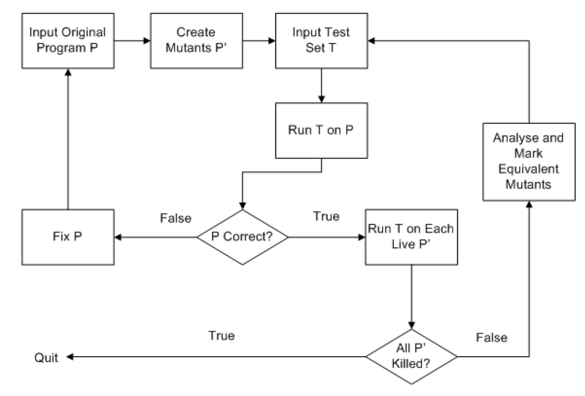
We start with the input program P in the upper left of the diagram. The first step, naturally, is to create mutants P' based on this program. The program must also be tested (a process orthogonal to the creation of mutants) on the test set T – note that we require a test set to already exist, an assumption noted in the previous section. If any errors are discovered while testing, we restart this process.
Now that we have a tested program with mutants P', we are able to run the test set on each live mutant – the qualifier of live here is so that we can kill mutants in future iterations of the loop without worrying about their impact on the test set. If all mutants are killed, then we conclude mutation testing for these mutants. If there are surviving mutants, on the other hand, we have more work to do. In particular, we need to evaluate if any of our mutants have found any “meaningful” errors (that is, they aren’t equivalent mutants, a property we will discuss later), and if so, update our test set T to have better coverage.
This control flow diagram we have just gone over underlies mutation testing as a whole. While the exact definitions of a program and test set may vary, mutation testing requires these stages to be evaluated in the order presented to be effective and work as mutation testing.
Core assumptions
Having built out our structure of how mutation testing works, it is perhaps a good time to establish why it actually works. Mutation testing theory relies fundamentally on two hypotheses: the coupling effect and the amusingly-named competent programmers hypothesis. To understand each, we will examine both the definition of and why each is important for making mutation testing work (at least theoretically).
Two papers [1] and [2] provide our reference definition for the coupling effect, namely that “a test data set that detects all simple faults in a program is so sensitive that it will also detect more complex faults”. This definition is notably “probabilistic rather than absolute” as stated in the same. To break this down a bit, consider a complicated error in a program, say a bug in how two structures interact. The coupling theory implies that a series of unit tests on the structures and their functions ought to be sufficient to catch this more complicated bug, at least probabilistically – notably, good code coverage helps with this property, since coverage can improve the test suite’s ability to catch possible errors.
The coupling effect is crucial to recovering interesting properties with mutation testing. Since mutation testing fundamentally works on small chunks of code, if not single operations, capturing the potential of complex interactions between objects or pieces of code requires that the coupling effect hold, at least some of the time. Additionally, test coverage, the main goal of mutation testing, is an interesting metric partly due to the coupling effect – in particular, if you provide sufficient test coverage, then you are more likely to catch errors in complex interactions.
Fortunately for the future of mutation testing, the coupling hypothesis has been well-tested both empirically and theoretically. These analyses specifically found that the coupling effect holds to a surprising degree in realistic applications, with one experiment indicating that tests developed to kill simple mutants killed 99 percent of more complicated mutants.
The competent programmer’s hypothesis (CPH) essentially states that programmers tend to produce code close to the stated goal. In particular, programmers tend to produce code that iteratively (if not monotonically) approaches what the solution should look like.
CPH is important for understanding the value of mutation testing – that programmers tend to get close to writing what they intend allows us to assume that tests will catch local but relevant errors to the correctness of the program. In turn, by mutating the underlying source code, we can simulate the likely errors that programmers will actually make, which allows mutation testing to provide insight into actual code variation. While there are few published results on the verified truth of CPH, I hope it is clear why this is a reasonable assumption to make in realistic settings.
Higher Order and Equivalent Mutants
Mutation testing theory is not just about single mutations that are applied to a codebase – we would also like to explore multiple mutations and the possibility that a mutation is equivalent to another mutation we can apply. These potential mutants are called higher order mutants and equivalent mutants, respectively. Each has important considerations and consequences for mutation testing theory.
Higher order mutants (HOMs) are broadly defined in the original paper to be the class of mutants that can be generated by changing more than a single operation / value in the source code. These HOMs can be generated in a variety of ways, including every combination of first-order mutations (note that first-order mutants are simply mutants that aren’t higher order). HOMs have the advantage of being potentially harder to kill (despite the coupling hypothesis, HOMs can sometimes require more information be gained from tests) and can catch potentially more interesting gaps in testing.
HOMs, specifically second-order mutants, have been found experimentally to improve coverage of issues found due to being more difficult to kill. This same experiment, however, also highlights the main risk of HOMs – without careful cost management techniques, HOMs can be much more expensive to generate than lower-order mutants. In particular, the complexity of the space covered by HOMs is much greater than first-order mutants, and are as such difficult to generate in a reasonable systematic way.
Equivalent mutants are defined to be mutants who have the exact same behavior as the program they were mutated from. This behavior is problematic, particularly when a mutant has the same behavior as the source code, since equivalent mutants are necessarily not killed. Proving that two programs are equivalent is of course impossible, but it is possible to evaluate if two programs are likely equivalent and avoid costly analysis of mutants that are ultimately meaningless.
For a concrete example of equivalent mutants, consider the mutants of the program demonstrated in part 1:
int foo_mutant2(int x) {
  return x * 1;
}
int foo_mutant3(int x) {
  return x + 0;
}
These two programs are “obviously” equivalent, but as noted, detecting this automatically is difficult at best and impossible in general. There are practical approaches to solving this problem, such as those illustrated in this paper. In short, these methods are able to find equivalent mutants with reasonable accuracy, practically reducing the probability of encountering an equivalent mutant in the wild.
In the final section of this article, we will examine some practical applications of mutation testing and some of the flaws of mutation testing as an approach.