k-nearest neighbors

Cornell CS 4/5780

Fall 2022

The k-NN algorithm

Assumption: Similar Inputs have similar outputs Classification rule: For a test input $\mathbf{x}$, assign the most common label amongst its k most similar training inputs

A binary classification example with $k=3$. The green point in the center is the test sample $\mathbf{x}$. The labels of the 3 neighbors are $2\times$(+1) and $1\times$(-1) resulting in majority predicting (+1).

Formal (and borderline incomprehensible) definition of k-NN:

Test point: $\mathbf{x}$

Denote the set of the $k$ nearest neighbors of $\mathbf{x}$ as $S_\mathbf{x}$. Formally $S_\mathbf{x}$ is defined as $S_\mathbf{x}\subseteq {D}$ s.t. $|S_\mathbf{x}|=k$ and $\forall(\mathbf{x}',y')\in D\backslash S_\mathbf{x}$, \[\text{dist}(\mathbf{x},\mathbf{x}')\ge\max_{(\mathbf{x}'',y'')\in S_\mathbf{x}} \text{dist}(\mathbf{x},\mathbf{x}''),\] (i.e. every point in $D$ but not in $S_\mathbf{x}$ is at least as far away from $\mathbf{x}$ as the furthest point in $S_\mathbf{x}$). We can then define the classifier $h()$ as a function returning the most common label in $S_\mathbf{x}$: \[h(\mathbf{x})=\text{mode}(\{y'':(\mathbf{x}'',y'')\in S_\mathbf{x}\}),\] where $\text{mode}(\cdot)$ means to select the label of the highest occurrence.

(Hint: In case of a draw, a good solution is to return the result of $k$-NN with smaller $k$.)

Quiz#1: How does $k$ affect the classifier? What happens if $k=n$? What if $k =1$?

What distance function should we use?

The k-nearest neighbor classifier fundamentally relies on a distance metric. The better that metric reflects label similarity, the better the classified will be. The most common choice is the Minkowski distance \[\text{dist}(\mathbf{x},\mathbf{z})=\left(\sum_{r=1}^d |x_r-z_r|^p\right)^{1/p}.\]
Quiz#2: This distance definition is pretty general and contains many well-known distances as special cases. Can you identify the following candidates?

$p = 1$:
$p = 2$:
$p \to \infty$:

The $k$NN classifier is still widely used today, but often with learned metrics. For more information on metric learning check out the Large Margin Nearest Neighbors (LMNN) algorithm to learn a pseudo-metric (nowadays also known as the triplet loss) or FaceNet for face verification.

Brief digression (Bayes optimal classifier)

Example: Assume (and this is almost never the case) you knew $\mathrm{P}(y|\mathbf{x})$, then you would simply predict the most likely label. \[ \text{The Bayes optimal classifier predicts:}\ y^* = h_\mathrm{opt}(\mathbf{x}) = \operatorname*{argmax}_y P(y|\mathbf{x}) \] Although the Bayes optimal classifier is as good as it gets, it still can make mistakes. It is always wrong if a sample does not have the most likely label. We can compute the probability of that happening precisely (which is exactly the error rate): $$\epsilon_{BayesOpt}=1-\mathrm{P}(h_\mathrm{opt}(\mathbf{x})|\mathbf{x}) = 1- \mathrm{P}(y^*|\mathbf{x})$$ Assume for example an email $\mathbf{x}$ can either be classified as spam $(+1)$ or ham $(-1)$. For the same email $\mathbf{x}$ the conditional class probabilities are: $$ \mathrm{P}(+1| \mathbf{x})=0.8\\ \mathrm{P}(-1| \mathbf{x})=0.2\\ $$ In this case the Bayes optimal classifier would predict the label $y^*=+1$ as it is most likely, and its error rate would be $\epsilon_{BayesOpt}=0.2$.

Why is the Bayes optimal classifier interesting, if it cannot be used in practice? The reason is that it provides a highly informative lower bound of the error rate. With the same feature representation no classifier can obtain a lower error. We will use this fact to analyze the error rate of the $k$NN classifier.

Briefer digression: Best constant predictor

While we are on the topic, let us also introduce an upper bound on the error --- i.e. a classifier that we will (hopefully) always beat. That is the constant classifier, which essentially predicts always the same constant independent of any feature vectors. The best constant in classification is the most common label in the training set. Incidentally, that is also what the $k$-NN classifier becomes if $k=n$. In regression settings, or more generally, the best constant is the constant that minimizes the loss on the training set (e.g. for the squared loss it is the average label in the training set, for the absolute loss the median label). The best constant classifier is important for debugging purposes -- you should always be able to show that your classifier performs significantly better on the test set than the best constant.

1-NN Convergence Proof

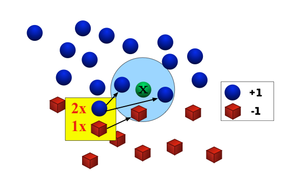
Cover and Hart 1967^[1]: As $n \to \infty$, the $1$-NN error is no more than twice the error of the Bayes Optimal classifier. (Similar guarantees hold for $k>1$.)

$n$ small

$n$ large

$n\to\infty$

Let $\mathbf{x}_\mathrm{NN}$ be the nearest neighbor of our test point $\mathbf{x}_\mathrm{t}$. As $n \to \infty$, $\text{dist}(\mathbf{x}_\mathrm{NN},\mathbf{x}_\mathrm{t}) \to 0$, i.e. $\mathbf{x}_\mathrm{NN} \to \mathbf{x}_{t}$. (This means the nearest neighbor is identical to $\mathbf{x}_\mathrm{t}$.) You return the label of $\mathbf{x}_\mathrm{NN}$. What is the probability that this is not the label of $\mathbf{x}_\mathrm{t}$? (This is the probability of drawing two different label of $\mathbf{x}$) \begin{multline*} \epsilon_{NN}=\mathrm{P}(y^* | \mathbf{x}_{t})(1-\mathrm{P}(y^* | \mathbf{x}_{NN})) + \mathrm{P}(y^* | \mathbf{x}_{NN})(1-\mathrm{P}(y^* | \mathbf{x}_{t}))\\ \le (1-\mathrm{P}(y^* | \mathbf{x}_{NN}))+(1-\mathrm{P}(y^* | \mathbf{x}_{t})) = 2(1-\mathrm{P}(y^* | \mathbf{x}_{t}) = 2\epsilon_\mathrm{BayesOpt}, \end{multline*} where the inequality follows from $\mathrm{P}(y^* | \mathbf{x}_{t})\le 1$ and $\mathrm{P}(y^* | \mathbf{x}_{NN})\le 1$. We also used that $\mathrm{P}(y^* | \mathbf{x}_{t})=\mathrm{P}(y^* | \mathbf{x}_{NN})$.

In the limit case, the test point and its nearest neighbor are identical. There are exactly two cases when a misclassification can occur: when the test point and its nearest neighbor have different labels. The probability of this happening is the probability of the two red events: $(1\!-\!p(s|\mathbf{x}))p(s|\mathbf{x})+p(s|\mathbf{x})(1\!-\!p(s|\mathbf{x}))=2p(s|\mathbf{x})(1-p(s|\mathbf{x}))$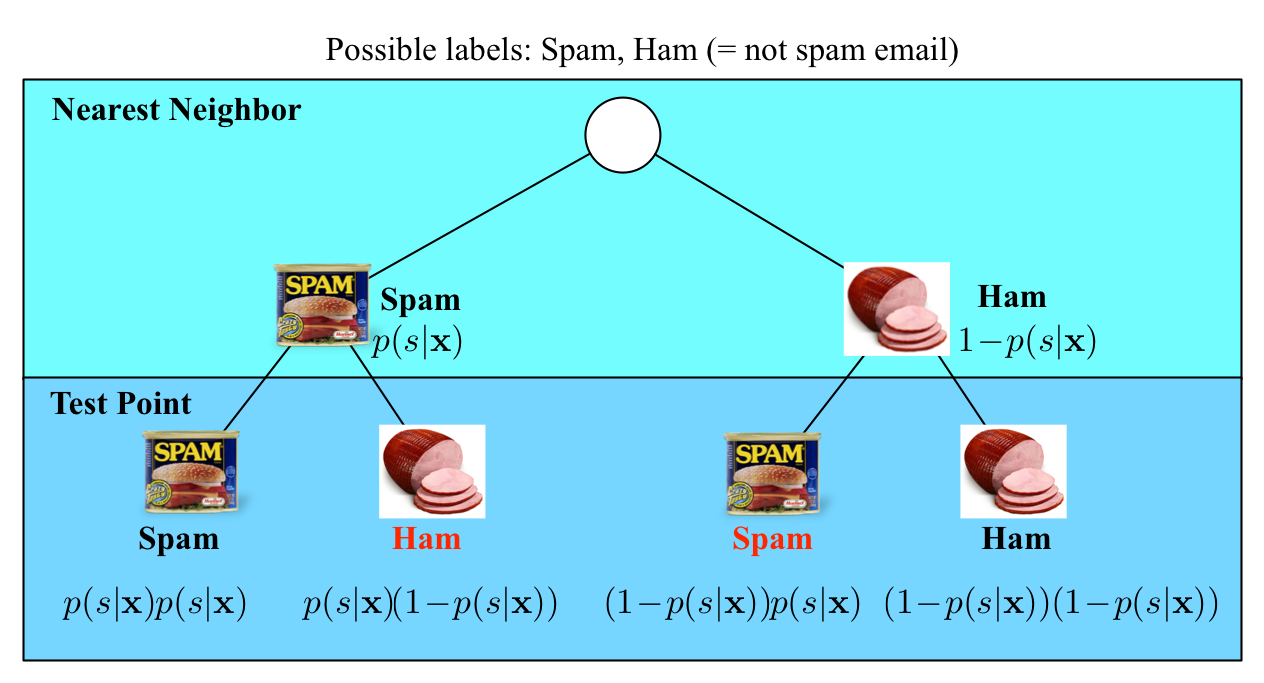

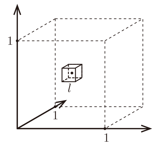
Good news: As $n \to\infty$, the $1$-NN classifier is only a factor 2 worse than the best possible classifier. Bad news: We are cursed!!

Curse of Dimensionality

Distances between points

The $k$NN classifier makes the assumption that similar points share similar labels. Unfortunately, in high dimensional spaces, points that are drawn from a probability distribution, tend to never be close together. We can illustrate this on a simple example. We will draw points uniformly at random within the unit cube (illustrated in the figure) and we will investigate how much space the $k$ nearest neighbors of a test point inside this cube will take up.

Formally, imagine the unit cube $[0,1]^d$. All training data is sampled uniformly within this cube, i.e. $\forall i, x_i\in[0,1]^d$, and we are considering the $k=10$ nearest neighbors of such a test point.

$d$		$\ell$
2		0.1
10		0.63
100		0.955
1000		0.9954

Let $\ell$ be the edge length of the smallest hyper-cube that contains all $k$-nearest neighbor of a test point. Then $\ell^d\approx\frac{k}{n}$ and $\ell\approx\left(\frac{k}{n}\right)^{1/d}$. If $n= 1000$, how big is $\ell$?

So as $d\gg 0$ almost the entire space is needed to find the $10$-NN. This breaks down the $k$-NN assumptions, because the $k$-NN are not particularly closer (and therefore more similar) than any other data points in the training set. Why would the test point share the label with those $k$-nearest neighbors, if they are not actually similar to it?

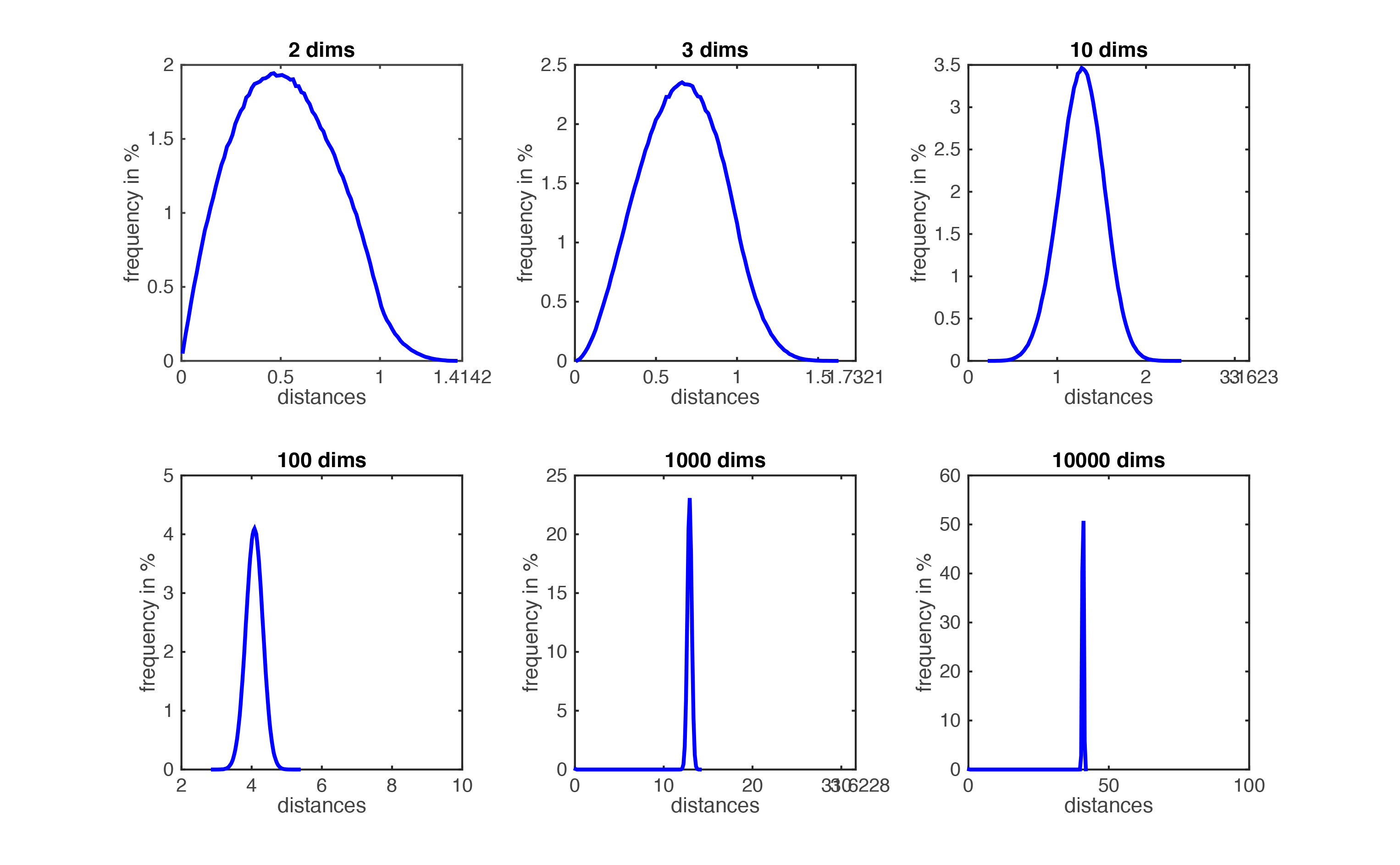
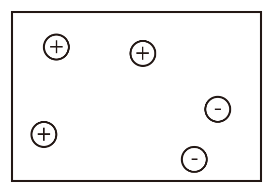
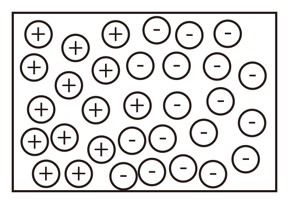
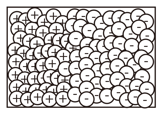
Figure demonstrating ``the curse of dimensionality''. The histogram plots show the distributions of all pairwise distances between randomly distributed points within $d$-dimensional unit squares. As the number of dimensions $d$ grows, all distances concentrate within a very small range.

One might think that one rescue could be to increase the number of training samples, $n$, until the nearest neighbors are truly close to the test point. How many data points would we need such that $\ell$ becomes truly small? Fix $\ell=\frac{1}{10}=0.1$ $\Rightarrow$ $n=\frac{k}{\ell^d}=k\cdot 10^d$, which grows exponentially! For $d>100$ we would need far more data points than there are electrons in the universe...

Distances to hyperplanes

So the distance between two randomly drawn data points increases drastically with their dimensionality. How about the distance to a hyperplane? Consider the following figure. There are two blue points and a red hyperplane. The left plot shows the scenario in 2d and the right plot in 3d. As long as $d=2$, the distance between the two points is $\sqrt{{\Delta x}^2+{\Delta y}^2}$. When a third dimension is added, this extends to $\sqrt{{\Delta x}^2+{\Delta y}^2+\Delta z^2}$, which must be at least as large (and is probably larger). This confirms again that pairwise distances grow in high dimensions. On the other hand, the distance to the red hyperplane remains unchanged as the third dimension is added. The reason is that the normal of the hyper-plane is orthogonal to the new dimension. This is a crucial observation. In $d$ dimensions, $d-1$ dimensions will be orthogonal to the normal of any given hyper-plane. Movement in those dimensions cannot increase or decrease the distance to the hyperplane --- the points just shift around and remain at the same distance. As distances between pairwise points become very large in high dimensional spaces, distances to hyperplanes become comparatively tiny. For machine learning algorithms, this is highly relevant. As we will see later on, many classifiers (e.g. the Perceptron or SVMs) place hyper planes between concentrations of different classes. One consequence of the curse of dimensionality is that most data points tend to be very close to these hyperplanes and it is often possible to perturb input slightly (and often imperceptibly) in order to change a classification outcome. This practice has recently become known as the creation of adversarial samples, whose existents is often falsely attributed to the complexity of neural networks.

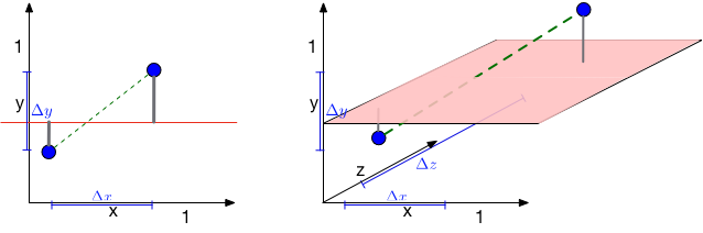
The curse of dimensionality has different effects on distances between two points and distances between points and hyperplanes.

An animation illustrating the effect on randomly sampled data points in 2D, as a 3rd dimension is added (with random coordinates). As the points expand along the 3rd dimension they spread out and their pairwise distances increase. However, their distance to the hyper-plane (z=0.5) remains unchanged --- so in relative terms the distance from the data points to the hyper-plane shrinks compared to their respective nearest neighbors.

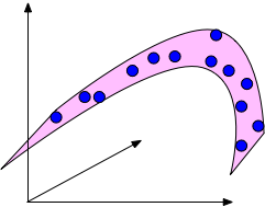
Data with low dimensional structure

However, not all is lost. Data may lie in low dimensional subspace or on sub-manifolds. Example: natural images (digits, faces). Here, the true dimensionality of the data can be much lower than its ambient space. The next figure shows an example of a data set sampled from a 2-dimensional manifold (i.e. a surface in space), that is embedded within 3d. Human faces are a typical example of an intrinsically low dimensional data set. Although an image of a face may require 18M pixels, a person may be able to describe this person with less than 50 attributes (e.g. male/female, blond/dark hair, ...) along which faces vary.

An example of a data set in 3d that is drawn from an underlying 2-dimensional manifold. The blue points are confined to the pink surface area, which is embedded in a 3-dimensional ambient space.

k-NN summary

$k$-NN is a simple and effective classifier if distances reliably reflect a semantically meaningful notion of the dissimilarity. (It becomes truly competitive through metric learning)
As $n \to \infty$, $k$-NN becomes provably very accurate, but also very slow.
As $d \gg 0$, points drawn from a probability distribution stop being similar to each other, and the $k$NN assumption breaks down.

Reference

[1]Cover, Thomas, and, Hart, Peter. Nearest neighbor pattern classification[J]. Information Theory, IEEE Transactions on, 1967, 13(1): 21-27