Fall 2022
In the first few lectures of this class we discussed supervised learning problems. While we will return to this setup soon, for this lecture and the next we will take a brief detour to discuss unsupervised learning. Colloquially, a key distinction from the supervised learning setup is that we now only have features \(x_1,\ldots,x_n\) (as usual, \(x_i\in\mathbb{R}^{d}\)) and no corresponding labels (in other words, no \(y_i\)). This means that in this setting we are not looking to make predictions. Instead, we are primarily interested in uncovering structure in the feature vectors themselves.
“Uncovering structure” is an admittedly vague concept and, more generally, the unsupervised learning problem tends to be more subjective then the supervised learning setup. Nevertheless, unsupervised learning is an important problem with applications such as data visualization, dimensionality reduction, grouping objects, exploratory data analysis, and more. Perhaps the most canonical example of unsupervised learning is clustering—given the \(n\) feature vectors we would like to group them into \(k\) collections based on similarity. For example, each feature vector \(x_i\) could represent a collection of movie ratings from user \(i\) and we would like to group the \(n\) users into sets of individuals with similar tastes in movies. We could then label the groups by examining the feature vectors (e.g., fans of historical dramas, animated films, or comedies), use the groupings to make recommendations, and even classify new users into existing groups. However, there is no ground truth taxonomy of movie watchers so we are never actually “predicting” a label and have no known baseline to compare with.
A key feature of the unsupervised learning problem is that the structure we find (if it exists) is intimately tied to the algorithm/methodology we choose. In this class we will primarily talk about two algorithms and, therefore, two types of structure we hope to uncover. First, we will explore how k-means clustering allows us to determine similar groups of feature vectors based on euclidean distances.1 Second, we will see how principal component analysis allows us to determine: (1) if the collection of features vectors lies in a lower dimensional space than their latent dimension \(d\) and (2) a small set of “synthetic” features that can be used to describe variability in the data.
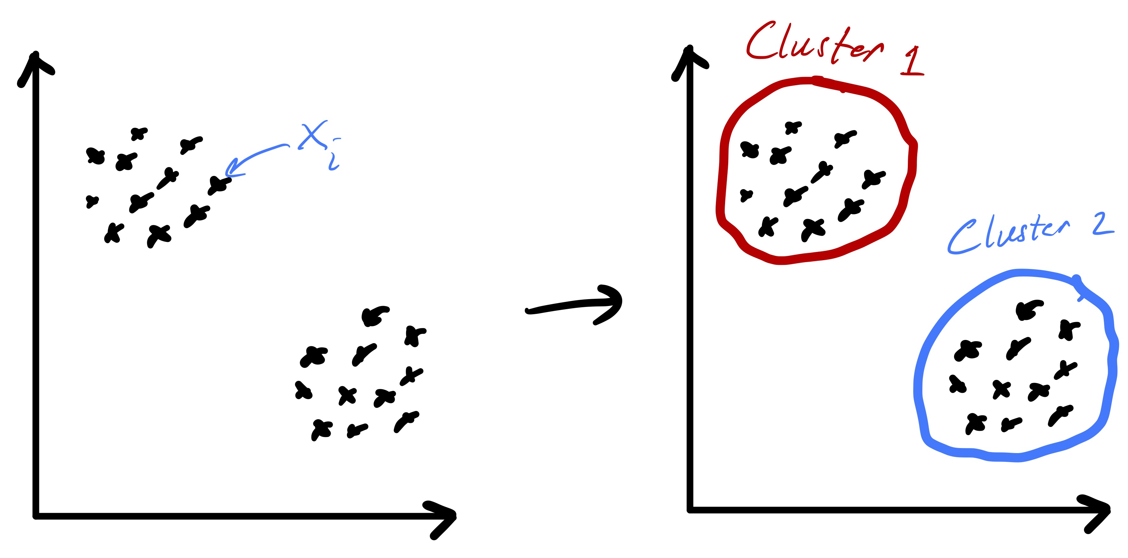
Given a set of \(n\) data points (i.e., feature vectors) \(x_1,\ldots,x_n\) with \(x_i\in\mathbb{R}^{d}\) the goal of k-means clustering is to partition the data into \(k\) groups2 where each group contains similar objects as defined by their euclidean distances.3 The ideal setting for such a procedure is readily illustrated in two dimensions by fig. 1.
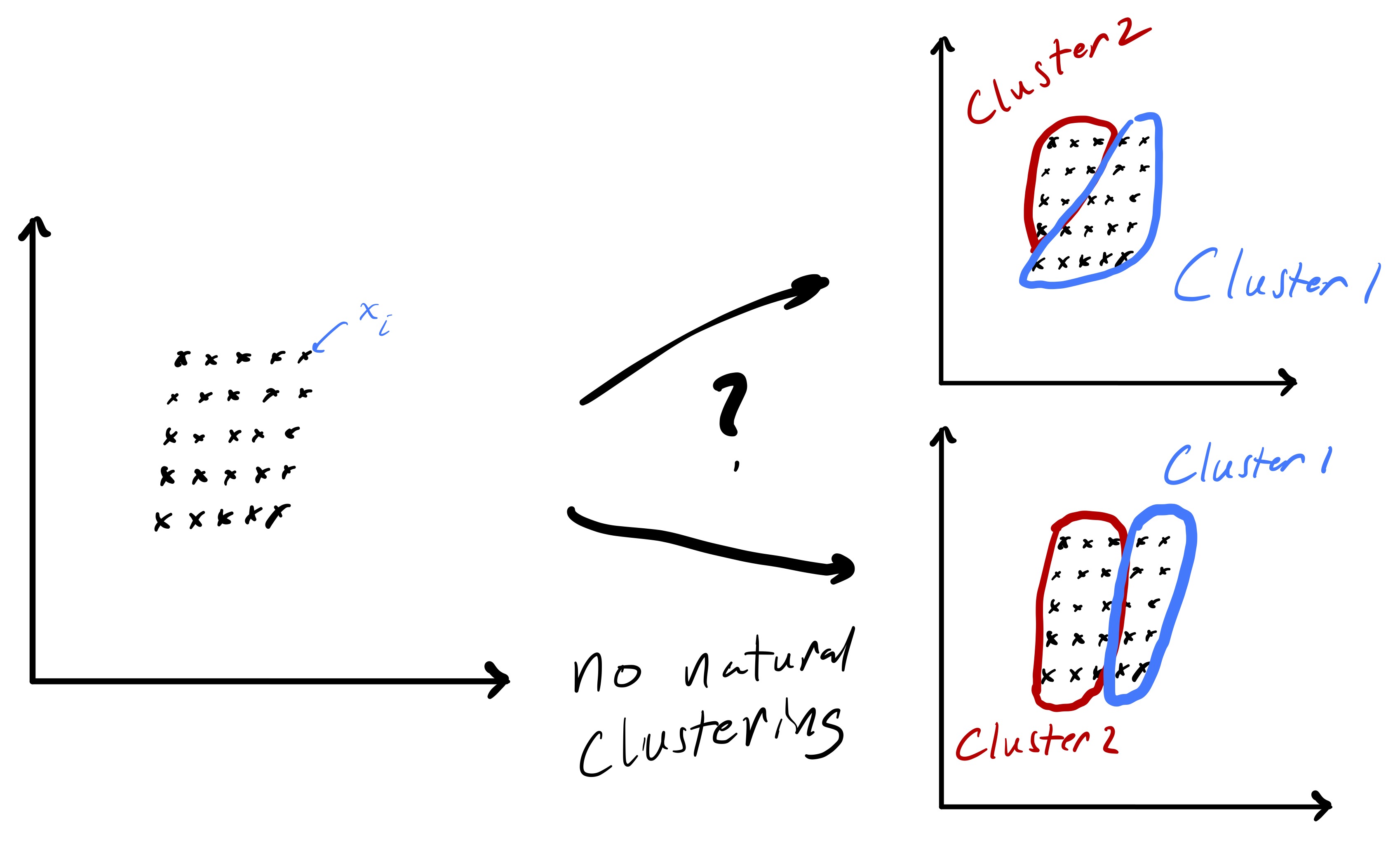
Importantly, fig. 1 started with points that lend themselves to a clustering based on euclidean distance—there were two clearly distinct sets of points. However, in the general setting we do not know that such a strategy will be effective a priori. While we will always be able to run the k-means algorithm presented here, there are data sets for which the resulting partition may be meaningless, e.g., as in fig. 2.
To formalize the clustering problem we need to introduce a bit of notation. Specifically, let the \(k\) subsets \(\mathcal{C}_{1},\ldots,\mathcal{C}_{k}\) with \(\mathcal{C}_{i} \subseteq \{1,\ldots,n\}\) specify the \(k\) clusters of points. In other words, if \(x_i\) is assigned to cluster \(j\) then \(i\in\mathcal{C}_j.\) To enforce that these subsets define a proper partition of the data we require that:
\(\bigcup_{i} \mathcal{C}_{i} = \{1,\ldots,n\}\) (I.e., every data point gets assigned to a cluster.)
\(\mathcal{C}_{i} \cap \mathcal{C}_{i'} = \emptyset\) for \(i\neq i'\) (I.e., the clusters do not overlap.)
We can now define what it means for a clustering to be “good.” Specifically, our aim will be to find clusters where the data points within each cluster are tightly grouped (i.e., exhibit low variability). Recall that \(\|x\|_ 2^2 = x^Tx,\) so \(\|x_i-x_j\|_ 2\) is the euclidean distance between the vectors \(x_i\) and \(x_j.\) Mathematically, for any cluster assignment we define \[ Z(\mathcal{C}_{1},\ldots,\mathcal{C}_{k}) = \sum_{\ell=1}^{k}\frac{1}{2\lvert\mathcal{C}_{\ell}\rvert} \sum_{i,j\in\mathcal{C}_{\ell}} \|x_{i} - x_{j}\|^{2}_ {2} \](1) and the smaller \(Z\) is, the better we consider the clustering. Roughly speaking, we are trying to pick a clustering that minimizes the pairwise squared distances within each cluster (normalized by the cluster sizes).
Interestingly, the definition of \(Z\) in eq. 1 can be rewritten in terms of the centroid of each cluster as \[ Z(\mathcal{C}_{1},\ldots,\mathcal{C}_{k}) = \sum_{\ell=1}^{k}\sum_{i\in\mathcal{C}_{\ell}} \|x_{i} - \mu_{\ell}\|^{2}_ {2}, \](2) where \[ \mu_{\ell} = \frac{1}{\lvert\mathcal{C}_{\ell}\rvert} \sum_{i\in\mathcal{C}_{\ell}} x_i \] is the mean/centroid of the points in cluster \(\ell.\) This formulation will be useful since it allows us to naturally think about the average of the points in a cluster as a center for the cluster. The algorithm we present later will actually use these centers to update clustering assignments.
Now that we have a formal way to define a good clustering of points, the ideal problem we would like to solve is \[ \min_{\mathcal{C}_{1},\ldots,\mathcal{C}_{k}} Z(\mathcal{C}_{1},\ldots,\mathcal{C}_{k}). \](3) Note that we have implicitly assumed we only consider \(\mathcal{C}_{i}\) that form valid partition and, therefore, have not explictly added those constraints. If we could efficiently solve this problem, then given \(k\) we could compute the ideal clustering of \(x_i\) into \(k\) groups (per our metric). Unfortunately, solving eq. 3 is not computationally feasible (in fact, there is a sense in which it is provably hard). Roughly speaking, we cannot do much better then simply trying all possible \(k\) way partitions of the data and seeing which one yields the smallest objective value. Nevertheless, while finding the minimizer of eq. 3 may be hard finding a good clustering is something we want to do in practice—to accomplish this we simply have to relax our goal of finding the “best” clustering.
The practical approach we will take finding a good clustering is to tackle eq. 3 via a local search algorithm. Given some initial clustering, we will iteratively update the cluster assignments in a manner that progressively yields a better and better clustering. However, the way in which we update the clusters will not ensure convergence to the global solution of our minimization problem. Instead, we will settle for a local solution—one where our update rule yields the same clusters we already have. The standard algorithm for solving the k-means clustering problem is known as Lloyd’s algorithm4 and is mathematically stated as:5
Input: data \(\{x_i\}_ {i=1}^{n}\) and \(k\)
Initialize \(C_{1},\ldots,C_{k}\)
While not converged:
- Compute \(\mu_{\ell} = \frac{1}{\lvert\mathcal{C}_{\ell}\rvert} \sum_{i\in\mathcal{C}_{\ell}} x_i\) for \(\ell=1,\ldots,k.\)
- Update \(\mathcal{C}_{1},\ldots,\mathcal{C}_{k}\) by assigning each data point \(x_i\) to the cluster whose centroid \(\mu_{\ell}\) it is closest to.
- If the cluster assignments didn’t change, we have converged.
Return: cluster assignments \(\mathcal{C}_{1},\ldots,\mathcal{C}_{k}\)
Fig. 3 demonstrates a procession of Lloyd’s algorithm (albeit somewhat inexactly since the cluster centroids are estimated). The key idea is that at each step we compute the centroid for each cluster and then reassign points to clusters based on which centroid they are closest too. This process actually has a nice feature that the objective function \(Z\) is non-increasing (and only fails to decrease if the cluster assignments have converged). Showing this fact is an interesting exercise (and may be an upcomming HW problem).
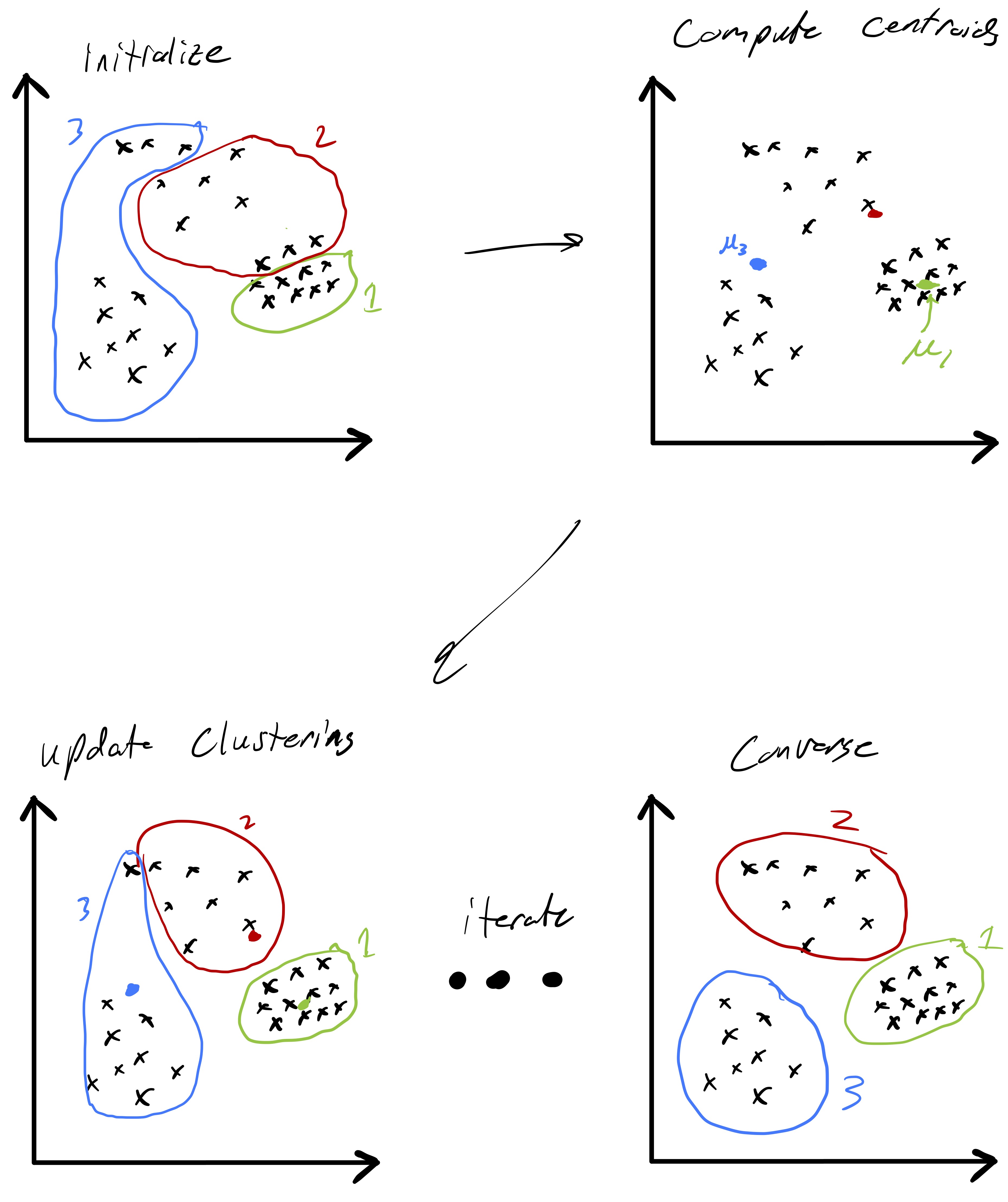
A more precise illustration is see in fig. 4 where data that seems to comprise of three clusters is given and the starting clustering is random. After picking an initial clustering, we find cluster centroids, reassign the points, and repeat till convergence. At each step the new cluster centroids are plotted as are the “dividing lines” that are used to assign points to clusters in the reassignment step. We will explain why these are linear later in the notes. At convergence we see that there is some ambiguity between the diffuse blue cluster and the yellow cluster near their boundary. This is partially due to the elongated ellipsoid structure of the data cluster to the right (that becomes the yellow cluster). Because we are using euclidean distances, we are making a modeling assumption that the clusters we want to find spread out roughly equally in all dimensions.

The cost of Lloyd’s algorithm is \(\mathcal{O}(ndk)\) per iteration and, therefore, in practice its efficiency is strongly dependent on how many iterations it takes to converge. While it is possible to estimate this in some special cases and develop worst case bounds, such specifics are beyond the scope of this course. It is also important to reiterate that Lloyd’s algorithm does not (necessarily) solve the optimization problem in eq. 3. As we will see in the next section, poor initial cluster assignments could result in convergence to a suboptimal clustering. One reason for this is that the cluster update steps are somewhat “local,” so if the ideal clustering looks very different than the current assignment the path Lloyd’s algorithm takes may not lead there.
While the k-means procedure is unsupervised, that does not mean it only takes data as input. In particular, there are two other choices the user has to make that can have a strong influence on the output. First, we have to decide how many clusters we want/expect, i.e., we have to choose \(k\). In some settings a natural choice for \(k\) may be evident based on some underlying knowledge about the data. However, in others it may be entirely unclear. Nevertheless, the choice of \(k\) can actually be quite important in many applications.
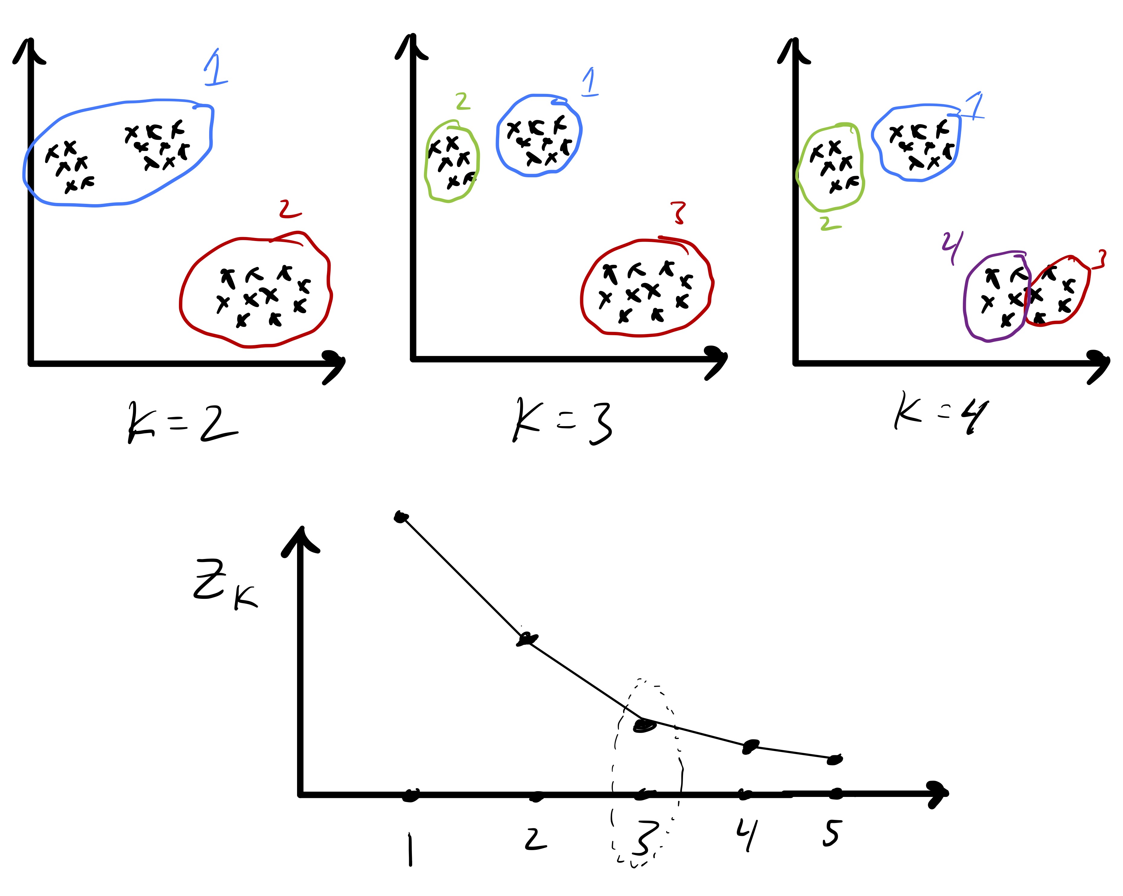
Because we have defined a measure of cluster quality, we can use that to help choose \(k.\) In particular, let \[ Z_k \equiv Z(\mathcal{C}_{1},\ldots,\mathcal{C}_{k}) \] be the computed objective value after we run Lloyd’s algorithm for some fixed value of \(k.\) Since \(Z_k\) measures the clustering quality we might be tempted to simply compute \(Z_1,Z_2,\ldots\) and simply pick \(k\) based on the the smallest value of \(Z_k.\) However, this is problematic because we expect the in-cluster variation to decrease naturally with \(k.\) In fact, \(Z_n = 0\) since every point is its own cluster. So, instead, we often look for the point at which \(Z_k\) stops decreasing quickly. The intuition is that as \(k\rightarrow k+1\) if a single big cluster naturally subdivides into two clear clusters we will see that \(Z_{k+1} \ll Z_{k}.\) In this case we may keep increasing \(k\) to see how the objective function further evolves. In contrast, if going from \(k\rightarrow k+1\) necessitates splitting up a clear cluster that does not naturally subdivide then we may see that \(Z_{k+1}\approx Z_{k}.\) An idealized version of this is illustrated in fig. 5. Once this, admittedly imprecise, criteria is met we may simply pick \(k\) as the number of clusters.
There are more rigorous ways to select \(k\) if we are willing to consider a null model for the data. For example, a common strategy is to consider the so-called gap statistic proposed by Tibshirani, Walther, and Hastie.6 In brief, this method compares the observed cluster variability \(Z_k\) to the expected variability if the data were uniformly distributed on a rectangle that contains the data. The number of clusters \(k\) is then chosen based on the comparisons of these metrics.
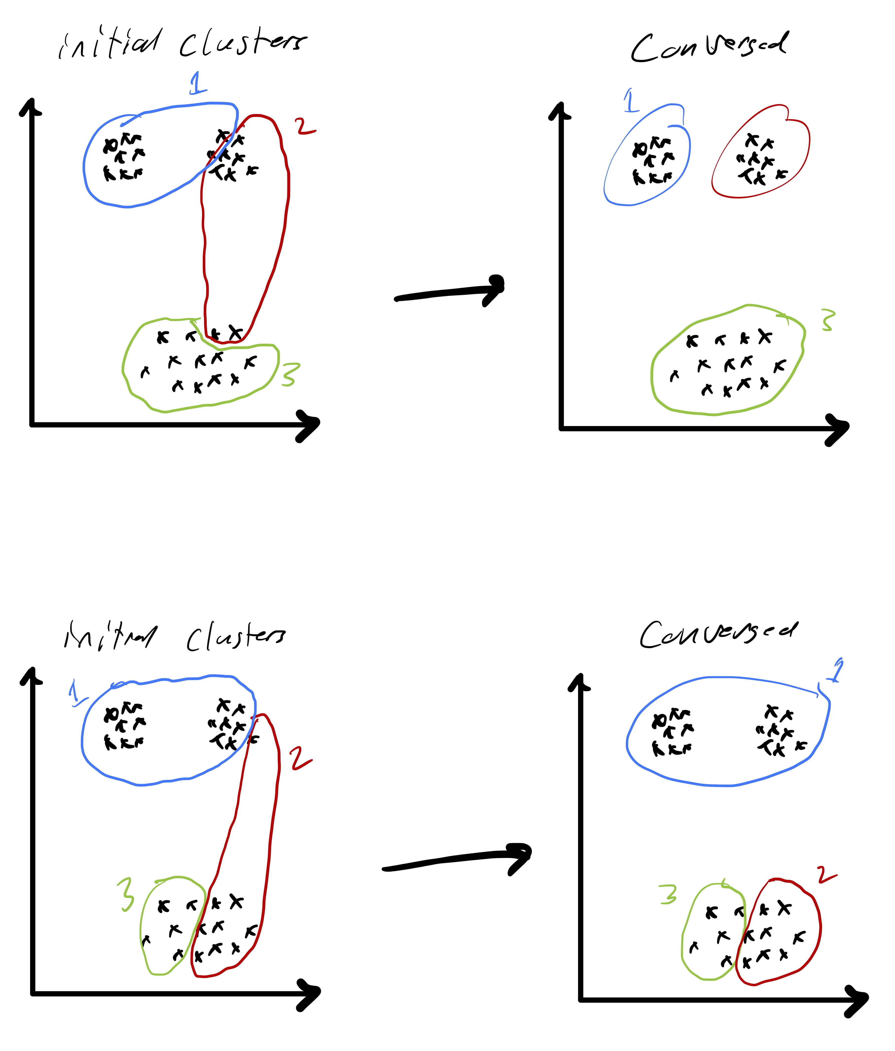
The second implicit input in Lloyd’s algorithm is an initial cluster assignment. This is particularly important because Lloyd’s algorithm only finds a local optima. So, very different initialization could result in convergence to very different solutions. An extreme version of this is in fig. 6 where one initialization yields a good solution and one yields a solution that is far from optimal. Because of this sensitivity, a common strategy is, for each \(k,\) to try several random initial clustering assignments.7 We then simply run Lloyd’s algorithm from each initial clustering and then take the output over those runs that yielded the smallest value of \(Z_k \equiv Z(\mathcal{C}_{1},\ldots,\mathcal{C}_{k}).\)
An alternative to thinking about initializing the cluster assignments is to randomly choose \(k\) cluster centers and then assign each point to the cluster center it is closest to (mirroring the assignment step in Lloyd’s algorithm). This perspective leads to one of the most common initialization strategies for k-means known as as k-means++.8 k-means++ uses data points themselves as the initial cluster centers and is based on the idea that the cluster centers should be somewhat spread out. To accomplish this, a data point is chosen uniformly at random and selected as a center. Subsequent centers are then chosen based on a distribution weighted by the distance to the closest already selected center. In this way, it is more likely to chose a well spaced out set of \(k\) data points to form the initial cluster centers. Details of this method are available in the aforementioned reference.
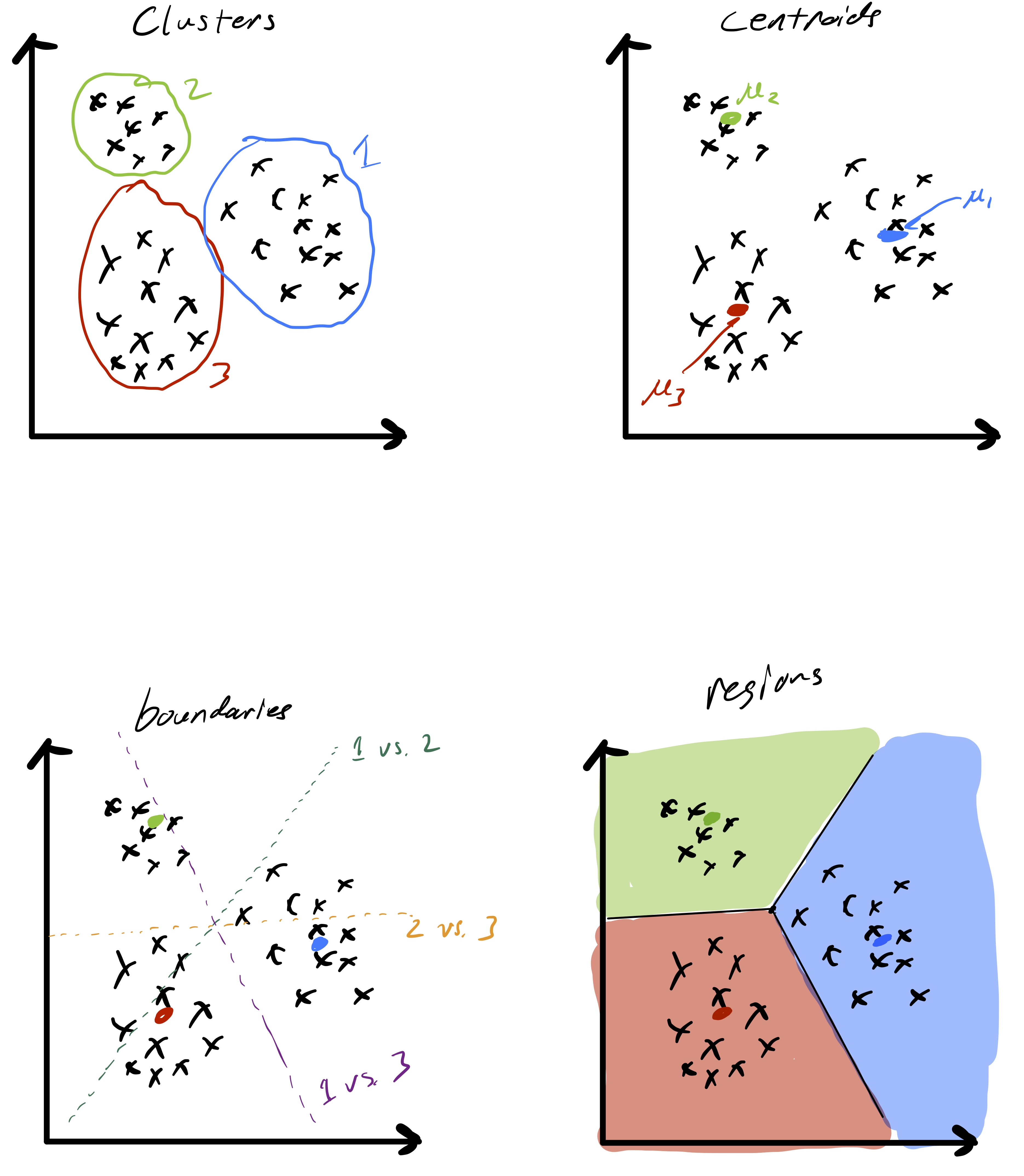
As alluded to, the unsupervised learning algorithm that we choose has a big impact on the type of structure we find in the data. In the case of k-means this structure can be readily described based on how cluster centroids partition \(\mathbb{R}^d\) when the cluster assignments are made. First, observe that given two cluster centroids \(\mu_{\ell}\) and \(\mu_{\ell'}\) the set of points equidistant from the two centroids defined as \(\{x\in\mathbb{R}^d \;\vert\; \|x-\mu_{\ell}\|_ 2 =\|x-\mu_{\ell'}\|_ 2\}\) is a line. This means that given a set of cluster centroids \(\mu_i,\ldots,\mu_k\) they implicitly partition space up into \(k\) domains whose boundaries are linear. Fig. 7 illustrates this point. Moreover, this shows how k-means is related to so-called Voronoi tessellations of space.
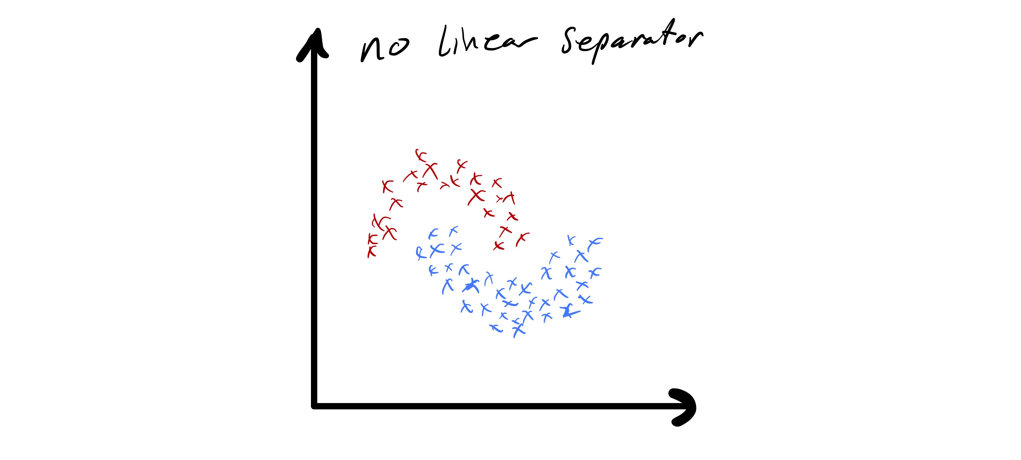
As we just observed, k-means clustering applied directly to the data \(x_i\in\mathbb{R}^{d}\) has some important limitations. In particular, the fact that cluster boundaries are necessarily linear can be quite limiting. In fig. 8 we see a data set that seems to nicely form a few clusters, but the boundaries between those clusters is quite clearly non-linear.
One approach to address this problem is known as spectral clustering.9 While the details of this approach (which has many variations) are outside the scope of this class, we provide a brief introduction to the method. The core idea behind spectral clustering is that the latent space where the data lives (for us, \(\mathbb{R}^d\)) is not the natural domain in which to perform k-means clustering. Therefore, we first perform a non-linear transform of the data.
Spectral clustering proceeds by first defining a similarity matrix \(A\in\mathbb{R}^{n\times n}\) where \(A_{i,j}\) provides some notion of similarity10 between \(x_i\) and \(x_j.\) For example, we could use a Gaussian similarity metric \(L_{i,j} = e^{-\|x_i-x_j\|_ 2^2/(2\sigma^2)}\) or a binary metric where \(A_{i,j} = 1\) if \(\|x_i-x_j\|_ 2 \leq \epsilon\) and \(0\) otherwise. Irrespective of the measure of similarity chosen, spectral clustering proceeds by forming the so-called Laplacian matrix \(L = D - A\) where \(D\) is a diagonal matrix and \(D_{i,i} = \sum_{j}A_{i,j}\). We then often let \(\hat{L}\) denote the normalized Laplacian matrix \(\hat{L} = I - D^{-1/2}AD^{-1/2}.\)
Given \(\hat{L}\) and \(k\) normalized spectral clustering11 proceeds as follows:
We have still used k-means and, therefore, linear decision boundaries to partition the \(v_i.\) However, by first performing an embedding of the data via the eigenvectors of \(\hat{L}\) this method allows for non-linear decision boundaries between clusters of \(x_i.\) The aforementioned references contains several examples where this proves effective.
Another important algorithm that is related to k-means clustering is fitting Gaussian mixture models via the expectation maximization (EM) algorithm. In this setting, we assume a generative model for the data \(x_i\) and try and fit parameters of that model to the given data. This has some benefits, e.g., it allows us to assign probabilities each point is in a given cluster, and reduces to k-means in a certain parameter regime. Moreover, even if the data are not actually drawn from a Gaussian mixture model it is possible to reason about the consequences of fitting such a model to the data; though, they are beyond the scope of this course.
In particular, here we will assume that the data points \(x_i\) are drawn from a mixture of \(k\) multivariate normal distributions each with their own means \(\mu_{\ell}\) and covariance matrices \(\Sigma_{\ell}\) for \(\ell=,\ldots,k\) and weighted by \(\pi_{\ell}.\) To be a proper mixture model we require that the vector \(\pi\in\mathbb{R}^k\) satisfies \(\pi_{\ell} \geq 0\) for \(\ell=1,\dots,k\) and \(\sum_{\ell}\pi_{\ell} = 1.\) We may now formally define the density of our mixture model \(\mathcal{M}(\pi,\mu_1,\ldots,\mu_k,\Sigma_1,\ldots,\Sigma_k)\) via \[ f(x) = \sum_{\ell} \pi_{\ell} \phi_{\ell}(x), \] where \(\phi_{\ell}\) is the density of \(\mathcal{N}(\mu_{\ell},\Sigma_{\ell}).\) Another way to think about this is that to draw a data point from the mixture model \(\mathcal{M}\) we first pick an integer from 1 to \(k\) based on the discrete density defined by \(\pi,\) say it is \(i,\) and then draw a sample from the multivariate normal distribution \(\mathcal{N}(\mu_{\ell},\Sigma_{\ell}).\)
If we knew which component of the mixture distribution (i.e., which normal distribution \(\mathcal{N}(\mu_{\ell},\Sigma_{\ell}\))$) generated each data point it would be a relatively simple problem to estimate the parameters of the individual mixture components (since we could just compute the MLE for \(\mu_{\ell}\) and \(\Sigma_{\ell}\) based on the data that came from that mixture component). However, our goal is a clustering of the data—if we knew this bit of information we would be done. Instead, given \(x_i\) we would like to estimate the probability it was generated by each of the mixture components. If we knew \(\pi\) and all the means and covariance matrices this would also be a simple calculation. The catch is that we have none of this information and have to simultaneously estimate the membership probabilities and the parameters of the mixture model. The membership probabilities will yield our “fuzzy” clustering of each data point into each of the \(k\) groups.
To formalize this let \(\Gamma\in\mathbb{R}^{n\times k}\) denote the membership probability of each data point \(x_i\) for each cluster (mixture component). Specifically, \(\Gamma_{i,\ell}\) will be the membership probability for \(x_i\) into mixture component \(\ell.\) Therefore, we require that \(\Gamma_{i,\ell}\geq 0\) and \(\sum_{\ell}\Gamma_{i,\ell} = 1.\) Given the parameters of the mixture model we can explicit compute the conditional probability that \(x_i\) was drawn from mixture component \(\ell\) as \[ \Gamma_{i,\ell} = \frac{\phi_{\ell}(x_i)\pi_{\ell}}{\sum_{j}\phi_{j}(x_i)\pi_j}. \]
We are now ready to present the EM algorithm; given data \(x_i\) as input and \(k\) it seeks to simultaneously compute membership probabilities and estimate mixture component parameters. Similar to the k-means algorithm it may only find a local optima of the underlying optimization problem (which we have omitted an explicit description of). This means that, as before, the output may be sensitive to the initialization and we are not guaranteed to find the mixture model that best describes the data. Lastly, determining convergence here is more subtle than in the case of k-means.
Input: data \(\{x_i\}_ {i=1}^{n}\) and \(k\)
Initialize \(\hat{\pi},\) means \(\hat{\mu}_1,\ldots,\hat{\mu}_{k}\) and covariance matrices \(\hat{\Sigma}_1,\ldots,\hat{\Sigma}_{k}\)
While not converged:
- Compute group membership probabilities \[ \Gamma_{i,\ell} = \frac{\phi_{\ell}(x_i)\pi_{\ell}}{\sum_{j}\phi_{j}(x_i)\pi_j}. \]
- Update mixture model parameters for \(\ell=1,\ldots,k\) as \[ \hat{\pi}_{\ell} = \frac{\sum_{i}\Gamma_{i,\ell}}{n} \] \[ \hat{\mu}_{\ell} = \frac{\sum_{i}\Gamma_{i,\ell}x_i}{\sum_{i}\Gamma_{i,\ell}} \] \[ \hat{\Sigma}_{\ell} = \frac{\sum_{i}\Gamma_{i,\ell}(x_i-\hat{\mu}_{\ell})(x_i-\hat{\mu}_{\ell})^T}{\sum_{i}\Gamma_{i,\ell}} \]
- Check for convergence
Return: Group membership probabilities \(\Gamma\) and mixture model parameter estimates \(\hat{\pi},\) \(\hat{\mu}_1,\ldots,\hat{\mu}_{k},\hat{\Sigma}_1,\ldots,\hat{\Sigma}_{k}\)
Typically, the two core steps of this algorithm are referred to as expectation steps and maximization steps. Step 1 is the expectation step where we compute conditional probabilities that represent group membership. Step 2 is then the maximization step where given a set of class membership probabilities we compute maximum likelihood estimates for the mixture model components. As before, there are several strategies to try and compute a good initialization for the necessary parameters.
If we return to the k-means algorithm it has a similar flavor. Assigning points based on the cluster centroids is analogous to the expectation step and updating the centroids is analogous to the maximization step. The connection can actually be made more explicit. In fact, we we restrict the covariance matrics to be \(\Sigma_{\ell} = \sigma^2 I\) and let \(\sigma \rightarrow 0\) the EM algorithm for a Gaussian mixture model essentially becomes the k-means algorithm.
Whereas k-means clustering sought to partition the data into homogeneous subgroups, principal component analysis (PCA) will seek to find, if it exists, low-dimensional structure in the data set \(\{x\}_ {i=1}^n\) (as before, \(x_i\in\mathbb{R}^d\)). This problem can be recast in several equivalent ways and we will see a few perspectives in these notes. Accordingly, PCA has many uses including data compression (analogous to building concise summaries of data points), item classification, data visualization, and more.
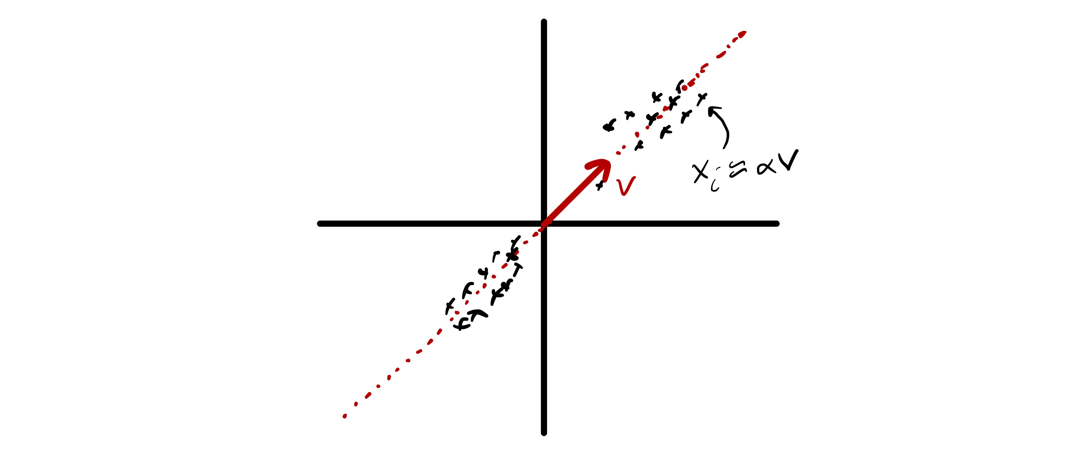
First, we will consider a simple mathematical model for data that directly motivates the PCA problem. Assume there exists some unit vector \(u\in\mathbb{R}^d\) such that \(x_i \approx \alpha_i u\) for some scalar \(\alpha_i.\)12 While \(x_i\) is high dimensional (assuming \(d\) is large), there is a sense in which it could be well approximated by a much smaller number of “features.” In fact, given \(u\) (which is the same for all \(x_i\)) we could well approximate our data using only \(n\) numbers—the \(\alpha_i.\) More concisely, we say that the \(x_i\) approximately lie in a subspace of dimension 1. Moreover, assuming the variability in \(\alpha_i\) is larger than whatever is hiding in the approximately equals above, just knowing the coefficients \(\alpha_i\) would also explain most of the variability in the data—if we want to understand how different various \(x_i\) are we could simply compare \(\alpha_i.\) This is illustrated in fig. 9, where we see two dimensional data that approximately lies in a one dimensional subspace.
More generally, we will describe PCA from two perspectives. First we will view PCA as finding a low-dimensional representation of the data that captures most of the interesting behavior. Here, “interesting” will be defined as variability. This is analogous to computing “composite” features (i.e., linear combinations of entries in each \(x_i\)) that explain most of the variability in the data. Second, we will see how PCA can be thought of as providing low-dimensional approximation to the data that is the best possible given the dimension (i.e., if we only allow ourselves \(k\) dimensions to represent \(d\) dimensional data we will do so in the best possible way).
Before proceeding with a mathematical formulation of PCA there is one important pre-processing step we need to perform on the data. Typically, in unsupervised learning we are interested in understanding relationships between data points and not necessarily bulk properties of the data.13 Taking the best approximation view of PCA this highlights a key problem of working with raw data points. In particular if the data has a sufficiently large mean, i.e., \(\mu = \frac{1}{n}\sum_i x_i\) is sufficiently far from zero, the best approximation of each data point is roughly \(\mu.\) An example of this is seen in fig. 10.
While finding \(\mu\) this tells us something about a data set, we know how to compute it and that is not the goal of PCA. Therefore, to actually understand the relationship between features we would like to omit this complication. Fortunately, this can be accomplished by centering our data before applying PCA. Specifically, we let \[
\hat{x}_ i = x_i - \mu,
\]
where \(\mu = \frac{1}{n}\sum_i x_i.\) We now simply work with the centered feature vectors \(\{\hat{x}_ i\}_ {i=1}^n\) and will do so throughout the remainder of these notes. Note that in some settings it may also be important to scale the entries of \(\hat{x}_ i\) (e.g., if they correspond to measurements that have vastly different scales).
The first goal we will use to describe PCA is finding a small set of composite features that capture most of the variability in the data. To illustrate this point, we will first consider finding a single composite feature that captures as much of the variability in the data set as possible. Mathematically, this corresponds to finding a vector \(\phi\in\mathbb{R}^d\) such that the sample variance of the scalars \[ z_i = \phi^T\hat{x}_ i \] is as large as possible.14 By convention we require that \(\|\phi\|_ 2 = 1,\) otherwise we could artificially inflate the variance by simply increasing the magnitude of the entries in \(\phi.\) Using the definition of sample variance we can now formally define the first principal component of a data set.
First principal component: The first principal component of a data set \(\{x_i\}_ {i=1}^n\) is the vector \(\phi\in\mathbb{R}^d\) that solves \[ \max_{\|\phi\|_ 2=1} \frac{1}{n}\sum_{i=1}^n(\phi^T\hat{x}_ i)^2. \](4)
When we discussed k-means above we framed it as an optimization problem and then discussed how actually solving that problem was hard. In this case we do not have such a complication—the problem in eq. 4 has a known solution. It is useful to introduce a bit more notation to state the solution. Specifically, we will consider the data matrix \[ \widehat{X}= \begin{bmatrix} \vert & & \vert \\ \hat{x}_ 1 & \cdots & \hat{x}_ n\\\vert & & \vert\end{bmatrix}. \] This allows us to rephrase eq. 4 as \[ \max_{\|\phi\|_ 2 =1}\|\hat{X}^T\phi\|_ 2. \] In other words, \(\phi\) is the unit vector that the matrix \(\widehat{X}^T\) makes as large as possible.
At this point we need to (re)introduce one of the most powerful matrix decompositions—the singular value decomposition (SVD).15 To simplify this presentation we make the reasonable assumption that \(n\geq d.\)16 In particular, we can always decompose the matrix \(\widehat{X}\) as \[ \widehat{X}= U\Sigma V^T \] where \(U\) is an \(d\times d\) matrix with orthonormal columns, \(V\) is an \(n\times d\) matrix with orthonormal columns, \(\Sigma\) is a \(d\times d\) diagonal matrix with \(\Sigma_{ii} = \sigma_i \geq 0,\) and \(\sigma_1 \geq \sigma_2 \geq \cdots \geq \sigma_d.\) Letting \[ U = \begin{bmatrix} \vert & & \vert \\ u_ 1 & \cdots & u_ d\\\vert & & \vert\end{bmatrix}, \quad V = \begin{bmatrix} \vert & & \vert \\ v_ 1 & \cdots & v_ d\\\vert & & \vert\end{bmatrix}, \quad \text{and} \quad \Sigma = \begin{bmatrix} \sigma_1 & & \\ & \ddots & \\& & \sigma_d \end{bmatrix} \] we call \(u_i\) the left singular vectors, \(v_i\) the right singular vectors, and \(\sigma_i\) the singular values. While methods for computing the SVD are beyond the scope of this class, efficient algorithms exist that cost \(\mathcal{O}(nd^2)\) and, in cases where \(n\) and \(d\) are large it is possible to efficiently compute only the first few singular values and vectors (e.g., for \(i=1,\ldots,k\)).
Under the mild assumption that \(\sigma_1 > \sigma_2\) the SVD the solution to eq. 4 becomes apparent: \(\phi = u_1.\)17 All \(\phi\) can be written as \(\phi = \sum_{i=1}^d a_i u_i\) where \(\sum_i a_i^2 = 1\) (because we want \(\|\phi\|_ 2=1\)). We now observe that \[ \begin{align} \|\widehat{X}^T\phi\|_ 2^2 &= \|V\Sigma U^T\phi\|_ 2^2 \\ & = \left\|\sum_{i=1}^d (\sigma_i a_i) v_i\right\|_ 2^2 \\ & = \sum_{i=1}^d (\sigma_i a_i)^2, \end{align} \] so the quantity is maximized by setting \(a_1=1\) and \(a_i = 0\) for \(i\neq 1.\)
So, the first left singular value of \(\widehat{X}\) gives us the first principal component of the data. What about finding additional directions? A natural way to set up this problem is to look for the composite feature with the next most variability. Informally, we could look for \(\psi\) such that \(y_i = \psi^T\hat{x}_ i\) has maximal sample variance. However, as stated we would simply get the first principal component again. Therefore, we need to force the second principal component to be distinct from this first. This is accomplished by forcing them to be orthogonal, i.e., \(\psi^T\phi = 0.\) While this may seem like a complex constraint it is actually not here. In fact, the SVD still reveals the solution: the second principal component is \(\psi=u_2.\) Fig. 11 illustrates how the first two principal components look for a stylized data set. We see that they reveal directions in which the data varies significantly.
More generally, we may want to consider the top \(k\) principal components. In other words the \(k\) directions in which the data varies the most. We denote the principal component \(\ell\) as \(\phi_{\ell}\) and to enforce that we find different directions we require that \(\phi_{\ell}^T\phi_{\ell'}^{\phantom{T}} = 0\) for \(\ell\neq\ell'.\) We also order them by the sample variance of \(\phi_{\ell}^T\hat{x}_ i,\) i.e., \(\phi_{\ell}^T\hat{x}_ i\) has greater variability than \(\phi_{\ell'}^T\hat{x}_ i\) for \(\ell < \ell'.\)
While we will not present a full proof, the SVD actually gives us all the principal components of the data set \(\{x_i\}_ {i=1}^n.\)
Principal components: Principal component \(\ell\) of data set \(\{x_i\}_ {i=1}^n\) is denoted \(\phi_{\ell}\) and satisfies \[ \phi_{\ell} = u_{\ell}, \]
where \(\widehat{X}= U\Sigma V^T\) is the SVD of \(\widehat{X}.\)
Our discussion of PCA started with considering variability in the data. Therefore, we would like to consider how the principal components explain variability in the data. First, by using the SVD of \(\widehat{X}\) we have already computed the sample variance for each principal component. In fact, we can show that \[ \text{Var}(\phi_{\ell}^T\hat{x}_ i) = \sigma_{\ell}^2/n. \] In other words, the singular values reveal the sample variance of \(\phi_{\ell}^T\hat{x}_ i.\)
Since we may want to think of principal components as providing a low-dimensional representation of the data a reasonable question to ask is how many we should compute/use for downstream tasks. One way to address this question is to try and address a sufficient fraction of the variability in the data. In other words, we pick \(k\) such that \(\phi_1,\ldots,\phi_k\) capture most of the variability in the data. To understand this we have to understand what the total variability of the data is. Fortunately, this is can be easily computed as \[ \sum_{j=1}^d\sum_{i=1}^n (\hat{x}_ i (j))^2. \] In other words we simply sum up the squares of all the entries in all the data points.
What is true, though less apparent, is that the total variability in the data is also encoded in the singular values of \(\widehat{X}\) since \[ \sum_{j=1}^d\sum_{i=1}^n (\hat{x}_ i (j))^2 = \sum_{i=1}^d \sigma_i^2. \] Similarly we can actually encode the total variability of the data captured by the first \(k\) principal components as \(\sum_{i=1}^k \sigma_i^2.\) (This is a consequence of the orthogonality of the principal components.) Therefore, the proportion of total variance explained by the first \(k\) principal components is \[ \frac{\sum_{i=1}^k \sigma_i^2}{\sum_{i=1}^d \sigma_i^2}. \] So, we can simply pick \(k\) to explain whatever fraction of the variance we want. Or, similar to with k-means we can pick \(k\) by identifying when we have diminishing returns in explaining variance by adding more principal components, i.e., looking for a knee in the plot of singular values.
We now briefly touch on how PCA is also solving a best approximation problem for the centered data \(\hat{x}_ i.\) Specifically, say we want to approximate every data point \(\hat{x}_ i\) by a point \(w_i\) in a fixed \(k\) dimensional subspace. Which subspace should we pick to minimize \(\sum_{i=1}^n \|\hat{x}_ i - w_i\|_ 2^2?\) Formally, this can be stated as finding a \(n\times k\) matrix \(W\) with orthonormal columns that solves \[ \min_{\substack{W\in\mathbb{R}^{n\times d}\\ \\ W^TW = I}} \sum_{i=1}^n \|\hat{x}_ i - W(W^T\hat{x}_ i)\|_ 2^2. \](5) This is because if we force \(w_i = Wz_i\) for some \(z_i\in\mathbb{R}^k\) (i.e., \(w_i\) lies in the span of the columns of \(W\)) the choice of \(z_i\) that minimizes \(\|\hat{x}_ i - Wz_i\|_ 2\) is \(z_i = W^T\hat{x}.\)
While this is starting to become a bit predictable, the SVD again yields the solution to this problem. In particular, the problem specified in eq. 5 is solved by setting the columns of \(W\) to be the first \(k\) left singular vectors of \(\widehat{X}\) or, analogously, the first \(k\) principal components. In other words, if we want to project our data \(\hat{x}_ i\) onto a \(k\) dimensional subspace the best choice is the subspace defined by the first \(k\) principal components. Notably, this fact is tied to our definition of best as the subspace where the sum of squared distances between the data points and their projections are minimized. The geometry of this is illustrated in fig. 12.
A common use of PCA is for data visualization. In particular, if we have high dimensional data that is hard to visualize we can sometimes see key features of the data by plotting its projection onto a few (1, 2, or 3) principal components. For example, if \(d=2\) this corresponds to forming a scatter plot of \((\phi_1^T\hat{x}_ i, \phi_2^T\hat{x}_ i).\) It is important to consider that only a portion of the variability in the data is “included” in visualizations of this type and any key information that is orthogonal to the first few principal components will be completely missed. Nevertheless, this way of looking at data can prove quite useful—see the class demo.
We will also briefly discuss how similar methods can be extended to incorporate “similarities” between features that are defined more generally than by \(\ell_2\) distance.↩︎
For the moment, assume \(k\) is given; we will return to this point later.↩︎
Much of this section could be written with a more general distance metric (e.g., \(\|\cdot\|_{1},\) \(\|\cdot\|_{\infty},\) or any well-defined metric \(d(\cdot,\cdot)\)). In fact, if we use \(\|\cdot\|_ {1}\) we recover an algorithm known as k-medians. However, in the general case it may not always be so easy to write down the appropriate update formula for the cluster assignments.↩︎
While Lloyd proposed the algorithm in 1957, an associated publication of his work did not appear till 1982 as Lloyd, S. P. “Least squares quantization in PCM” IEEE Transactions on Information Theory 28 (2), 129–137, (1982).↩︎
Some aspects of this algorithm may seem under specified—we will get to them later.↩︎
See Tibshirani R., Walther G., and Hastie T. “Estimating the number of clusters in a data set via the gap statistic” J. R. Statist. Soc. B 63 (2), 411-423, (2001).↩︎
There are many ways to assign an initial clustering “at random.” For example, for each data point we could independently assign it to a cluster uniformly at random (i.e., point \(x_i\) ends up in cluster \(\ell\) w.p. \(1/k\)).↩︎
See Arthur, D. and Vassilvitskii, S. “k-means++: the advantages of careful seeding” Proceedings of the eighteenth annual ACM-SIAM symposium on Discrete algorithms, 1027–1035, (2007).↩︎
One good resource to learn more is Von Luxburg, U. “A tutorial on spectral clustering.” Statistics and computing 17 (4), 395-416, 2007. A version is available on arXiv.↩︎
We do require that \(A_{i,j} \geq 0\) and \(A_{i,j} = A_{j,1}.\)↩︎
See Ng, A.Y., Jordan, M.I. and Weiss, Y., “On spectral clustering: Analysis and an algorithm,”” In Advances in neural information processing systems 849-856, 2002.↩︎
Assume that the error in this approximation is much smaller than the variation in the coefficients \(\alpha_i.\)↩︎
For example, k-means is shift invariant—if we add an arbitrary vector \(w\in\mathbb{R}^d\) to every data point it does not change the outcome of our algorithm/analysis.↩︎
We call this a composite feature because \(z_i\) is a linear combinantion of the features (entries) in each data vector \(\hat{x}_ i.\)↩︎
This is often taught using eigenvectors instead. The connection is through the sample covariance matrix \(\widehat{\Sigma} = \widehat{X}\widehat{X}^T.\) The singular vectors we will use are equivalent to the eigenvectors of \(\widehat{\Sigma}\) the the eigenvalues of \(\widehat{\Sigma}\) are the singular values of \(\widehat{X}\) squared.↩︎
Everything works out fine if \(n< d\) but we need to write \(\min(n,d)\) in a bunch of places.↩︎
If \(\sigma_1 = \sigma_2\) the first principal component is not well defined.↩︎