$$
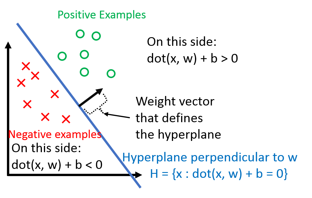
h(x_i) = \textrm{sign}(\mathbf{w}^\top \mathbf{x}_i + b)
$$
\(b\) is the bias term (without the bias term, the hyperplane that \(\mathbf{w}\) defines would always have to go through the origin).
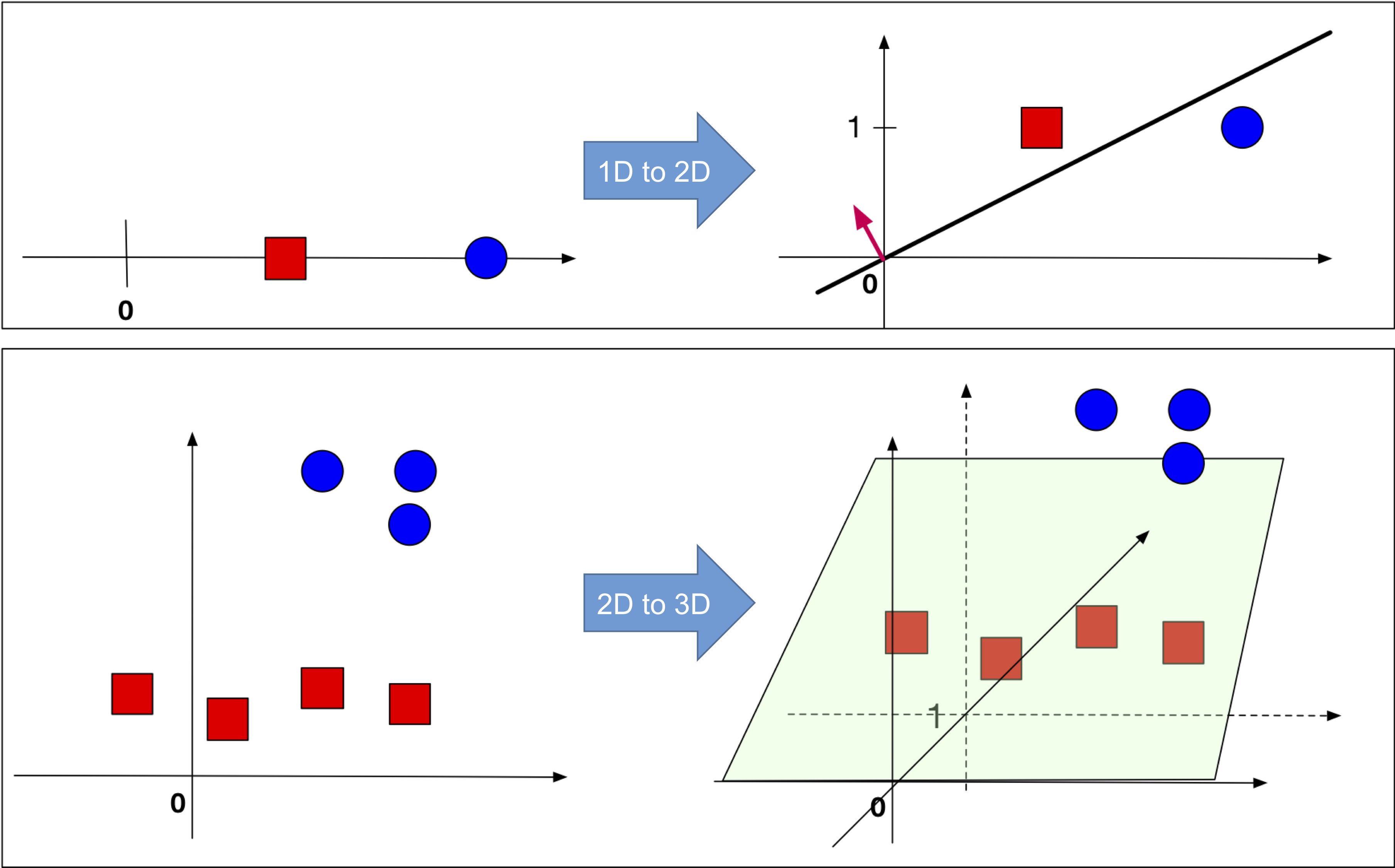
Dealing with \(b\) can be a pain, so we 'absorb' it into the feature vector \(\mathbf{w}\) by adding one additional constant dimension.
Under this convention,
$$
\mathbf{x}_i \hspace{0.1in} \text{becomes} \hspace{0.1in} \begin{bmatrix} \mathbf{x}_i \\ 1 \end{bmatrix} \\
\mathbf{w} \hspace{0.1in} \text{becomes} \hspace{0.1in} \begin{bmatrix} \mathbf{w} \\ b \end{bmatrix} \\
$$
We can verify that
$$
\begin{bmatrix} \mathbf{x}_i \\ 1 \end{bmatrix}^\top \begin{bmatrix} \mathbf{w} \\ b \end{bmatrix} = \mathbf{w}^\top \mathbf{x}_i + b
$$
Using this, we can simplify the above formulation of \(h(\mathbf{x}_i)\) to
$$
h(\mathbf{x}_i) = \textrm{sign}(\mathbf{w}^\top \mathbf{x})
$$
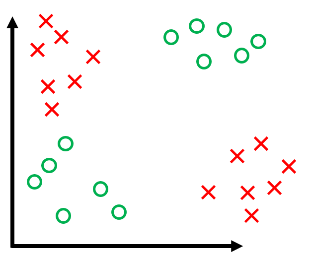
(Left:) The original data is 1-dimensional (top row) or 2-dimensional (bottom row). There is no hyper-plane that passes through the origin and separates the red and blue points. (Right:) After a constant dimension was added to all data points such a hyperplane exists.
Observation: Note that
$$
y_i(\mathbf{w}^\top \mathbf{x}_i) > 0 \Longleftrightarrow \mathbf{x}_i \hspace{0.1in} \text{is classified correctly}
$$
where 'classified correctly' means that \(x_i\) is on the correct side of the hyperplane defined by \(\mathbf{w}\).
Also, note that the left side depends on \(y_i \in \{-1, +1\}\) (it wouldn't work if, for example \(y_i \in \{0, +1\}\)).
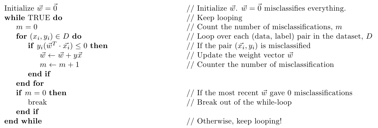
Perceptron Algorithm
Now that we know what the \(\mathbf{w}\) is supposed to do (defining a hyperplane the separates the data), let's look at how we can get such \(\mathbf{w}\).
Perceptron Algorithm
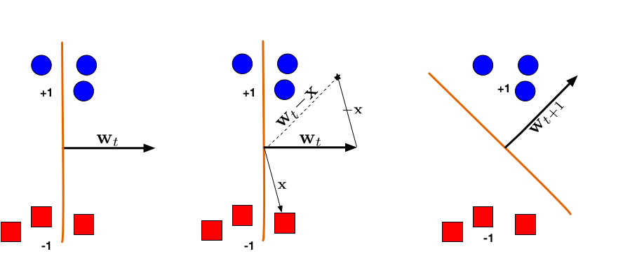
Geometric Intuition
Illustration of a Perceptron update. (Left:) The hyperplane defined by \(\mathbf{w}_t\) misclassifies one red (-1) and one blue (+1) point. (Middle:) The red point \(\mathbf{x}\) is chosen and used for an update. Because its label is -1 we need to subtract \(\mathbf{x}\) from \(\mathbf{w}_t\). (Right:) The udpated hyperplane \(\mathbf{w}_{t+1}=\mathbf{w}_t-\mathbf{x}\) separates the two classes and the Perceptron algorithm has converged.
Quiz: Assume a data set consists only of a single data point \(\{(\mathbf{x},+1)\}\). How often can a Perceptron misclassify this point \(\mathbf{x}\) repeatedly? What if the initial weight vector \(\mathbf{w}\) was initialized randomly and not as the all-zero vector?
Perceptron Convergence
The Perceptron was arguably the first algorithm with a strong formal guarantee. If a data set is linearly separable, the Perceptron will find a separating hyperplane in a finite number of updates. (If the data is not linearly separable, it will loop forever.)
The argument goes as follows:
Suppose \(\exists \mathbf{w}^*\) such that \(y_i(\mathbf{x}^\top \mathbf{w}^* ) > 0 \) \(\forall (\mathbf{x}_i, y_i) \in D\).
Now, suppose that we rescale each data point and the \(\mathbf{w}^*\) such that
$$
||\mathbf{w}^*|| = 1 \hspace{0.3in} \text{and} \hspace{0.3in} ||\mathbf{x}_i|| \le 1 \hspace{0.1in} \forall \mathbf{x}_i \in D
$$
Let us define the Margin \(\gamma\) of the hyperplane \(\mathbf{w}^*\) as
\(
\gamma = \min_{(\mathbf{x}_i, y_i) \in D}|\mathbf{x}_i^\top \mathbf{w}^* |
\).
A little observation (which will come in very handy): For all \(\mathbf{x}\) we must have \(y(\mathbf{x}^\top \mathbf{w}^*)=|\mathbf{x}^\top \mathbf{w}^*|\geq \gamma\). Why? Because \(\mathbf{w}^*\) is a perfect classifier, so all training data points \((\mathbf{x},y)\) lie on the "correct" side of the hyper-plane and therefore \(y=sign(\mathbf{x}^\top \mathbf{w}^*)\). The second inequality follows directly from the definition of the margin \(\gamma\).
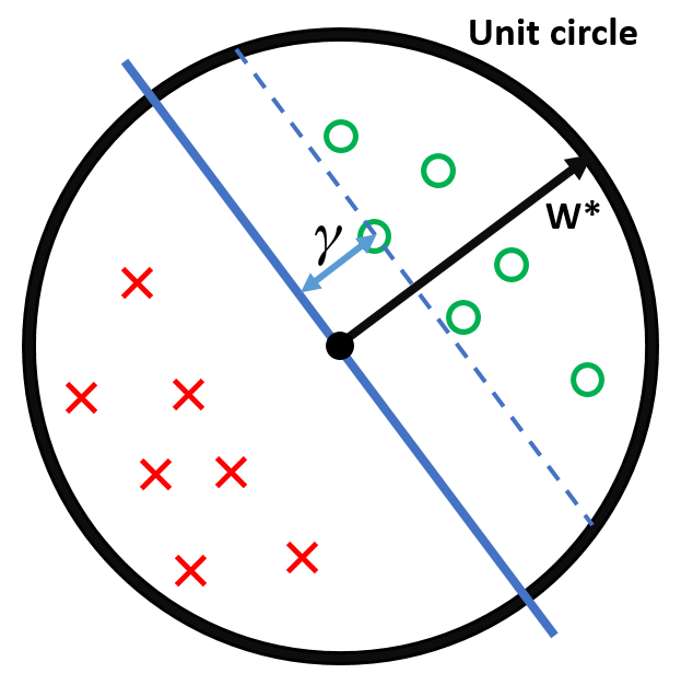
To summarize our setup:
All inputs \(\mathbf{x}_i\) live within the unit sphere
There exists a separating hyperplane defined by \(\mathbf{w}^*\), with \(\|\mathbf{w}\|^*=1\) (i.e. \(\mathbf{w}^*\) lies exactly on the unit sphere).
\(\gamma\) is the distance from this hyperplane (blue) to the closest data point.
Theorem: If all of the above holds, then the Perceptron algorithm makes at most \(1 / \gamma^2\) mistakes.
Proof:
Keeping what we defined above, consider the effect of an update (\(\mathbf{w}\) becomes \(\mathbf{w}+y\mathbf{x}\)) on the two terms \(\mathbf{w}^\top \mathbf{w}^*\) and \(\mathbf{w}^\top \mathbf{w}\).
We will use two facts:
\(y( \mathbf{x}^\top \mathbf{w})\leq 0\): This holds because \(\mathbf x\) is misclassified by \(\mathbf{w}\) - otherwise we wouldn't make the update.
\(y( \mathbf{x}^\top \mathbf{w}^*)>0\): This holds because \(\mathbf{w}^*\) is a separating hyper-plane and classifies all points correctly.
Consider the effect of an update on \(\mathbf{w}^\top \mathbf{w}^*\):
$$
(\mathbf{w} + y\mathbf{x})^\top \mathbf{w}^* = \mathbf{w}^\top \mathbf{w}^* + y(\mathbf{x}^\top \mathbf{w}^*) \ge \mathbf{w}^\top \mathbf{w}^* + \gamma
$$
The inequality follows from the fact that, for \(\mathbf{w}^*\), the distance from the hyperplane defined by \(\mathbf{w}^*\) to \(\mathbf{x}\) must be at least \(\gamma\) (i.e. \(y (\mathbf{x}^\top \mathbf{w}^*)=|\mathbf{x}^\top \mathbf{w}^*|\geq \gamma\)).
This means that for each update, \(\mathbf{w}^\top \mathbf{w}^*\) grows by at least \(\gamma\).
Consider the effect of an update on \(\mathbf{w}^\top \mathbf{w}\):
$$
(\mathbf{w} + y\mathbf{x})^\top (\mathbf{w} + y\mathbf{x}) = \mathbf{w}^\top \mathbf{w} + \underbrace{2y(\mathbf{w}^\top\mathbf{x})}_{<0} + \underbrace{y^2(\mathbf{x}^\top \mathbf{x})}_{0\leq \ \ \leq 1} \le \mathbf{w}^\top \mathbf{w} + 1
$$
The inequality follows from the fact that
\(2y(\mathbf{w}^\top \mathbf{x}) < 0\) as we had to make an update, meaning \(\mathbf{x}\) was misclassified
\(0\leq y^2(\mathbf{x}^\top \mathbf{x}) \le 1\) as \(y^2 = 1\) and all \(\mathbf{x}^\top \mathbf{x}\leq 1\) (because \(\|\mathbf x\|\leq 1\)).
This means that for each update, \(\mathbf{w}^\top \mathbf{w}\) grows by at most 1.
Now remember from the Perceptron algorithm that we initialize \(\mathbf{w}=\mathbf{0}\). Hence, initially \(\mathbf{w}^\top\mathbf{w}=0\) and \(\mathbf{w}^\top\mathbf{w}^*=0\) and after \(M\) updates the following two inequalities must hold:
(1) \(\mathbf{w}^\top\mathbf{w}^*\geq M\gamma\)
(2) \(\mathbf{w}^\top \mathbf{w}\leq M\).
We can then complete the proof:
\begin{align}
M\gamma &\le \mathbf{w}^\top \mathbf{w}^* &&\text{By (1)} \\
&=\|\mathbf{w}\|\cos(\theta) && \text{by definition of inner-product, where \(\theta\) is the angle between \(\mathbf{w}\) and \(\mathbf{w}^*\).}\\
&\leq ||\mathbf{w}|| &&\text{by definition of \(\cos\), we must have \(\cos(\theta)\leq 1\).} \\
&= \sqrt{\mathbf{w}^\top \mathbf{w}} && \text{by definition of \(\|\mathbf{w}\|\)} \\
&\le \sqrt{M} &&\text{By (2)} \\
& \textrm{ }\\
&\Rightarrow M\gamma \le \sqrt{M} \\
&\Rightarrow M^2\gamma^2 \le M \\
&\Rightarrow M \le \frac{1}{\gamma^2} && \text{And hence, the number of updates \(M\) is bounded from above by a constant.}
\end{align}
Quiz: Given the theorem above, what can you say about the margin of a classifier (what is more desirable, a large margin or a small margin?) Can you characterize data sets for which the Perceptron algorithm will converge quickly? Draw an example.