Chapter 7 Traffic Network Games

In this chapter, we return to traffic flows, but this time we consider them in a game-theoretic context.

7.1 Definition of a Traffic Network Game

Consider a scenario where players want to travel on graph $G$ from a starting node $s$ to a destination $t$ ; each edge in $G$ is associated with some travel time that may depend on the number of players that traverse the edge, and the total travel time incurred to a player is the sum of the travel times of all the edges it traverses. The players are participating in a game where they need to decide what $(s, t)$ -path to take in $G$ , and their goal is to minimize their total travel time. In more detail, a traffic network game $𝒢$ on a directed graph $G = (V, E)$ is specified as follows:

We associate with each edge

e \in E

, a travel time function

T_{e} (\cdot)

, which determines the travel time

T_{e} (x)

on the “road”

e

x

players are traveling on it.

We assume the travel time is linear:

T_{e} (x) = α_{e} x + β_{e}

, where

α_{e}, β_{e} \geq 0

. (So, the more people are traveling on an edge, the longer it should take.)

We specify a source

s \in V

and a sink

t \in V

; the goal of all players is to travel from

s

t

. The action set for each player is the set of paths

p

from

s

t

An outcome (action profile)

\vec{p}

thus specifies a path for each player.

In such an outcome

\vec{p}

, let

x_{e} (\vec{p})

denote the number of players traveling on edge

e

in that outcome.

Each player $i$ ’s utility is defined as the negative of their travel time: $u_{i} (\vec{p}) = - \sum_{e \in p_{i}} T_{e} (x_{e} (\vec{p})) .$
(The reason we take the negative of the travel time is so that longer travel times are considered less desirable.)

More formally,

Definition 7.1. We refer to the tuple $(G = (V, E), {α_{e}, β_{e}}_{e \in E}, s, t)$ where $G$ is a directed graph, $(s, t)$ a source-sink pair in $G$ , and for all $e \in E$ , $α_{e}, β_{e} \in ℝ_{\geq 0}$ , as a traffic network problem. The traffic network game $𝒢 = (n, A, \vec{u})$ corresponding to the traffic network problem $(G = (V, E), {α_{e}, β_{e}}_{e \in E}, s, t)$ is defined as follows:

For each player $i$ , let $A_{i}$ be the set of $(s, t)$ -paths in $G$ .
For each player $i$ , let $u_{i} (\vec{p}) = - \sum_{e \in p_{i}} T_{e} (x_{e} (\vec{p})),$
where $T_{e} (x) = α_{e} x + β_{e}$ and $x_{e}$ is the number of players traveling on the edge $e$ in the outcome $\vec{p}$ .

Example 7.1. Consider the traffic network in the left of Figure 7.1 with 4,000 players traveling from $A$ to $B$ , where there are four edges; $(A, C), (D, B)$ have travel time $T_{(A, C)} (x) = T_{(D, B)} (x) = \frac{x}{100}$ , and $(C, B)$ and $(A, D)$ have travel time $T_{(C, B)} (x) = T_{(A, D)} (x) = 45$ . There are only two possible paths from $A$ to $B$ , and thus only two possible actions for the players: let us call them $Up$ ( $A \to C \to B$ ) and Down ( $A \to D \to B$ ). If everyone goes $Up$ , then the travel time for everyone is $40 + 45 = 85$ ; the same applies if everyone goes Down.

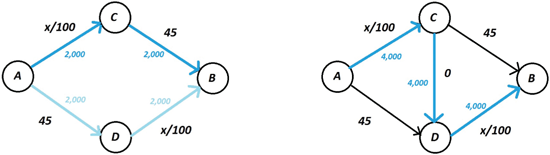
**Figure 7.1:** *Left*: A basic example of a traffic network game. The label in black represents the travel time on the edge, and the label in blue represents the number of players traveling on the edge in the PNE. *Right*: How the PNE changes when we add a “highway” from $C$ to $D$ .

But if half go Up and half go Down, everyone gets a travel time of $20 + 45 = 65$ . This is, in fact, the unique PNE for this game—if more than half of the players are traveling along one of the two paths, a player traveling on that path can decrease their travel time by switching to the other path.

7.2 Braess’s Paradox

Consider again the network on the left in Figure 7.1, but let us augment it by adding an extremely efficient road from $C$ to $D$ with travel time 0 (no matter how many people travel on it), resulting in the network on the right in Figure 7.1. Intuitively, we would think that adding such an amazing new road would decrease the travel time for everyone. Surprisingly, the opposite happens!

Note that we have added a new path (i.e., action), $A \to C \to D \to B$ , to the game; let us call this action $Highway$ . There is again a unique PNE in the game, and it is one where everyone plays $Highway$ , which leads to the travel time increasing to $40 + 40 = 80$ ! In fact, $Highway$ is a strictly dominant action (and thus the only PNE): the segment $A \to C$ is a strictly better than $A \to D$ (even if everyone travels on $A \to C$ ), and $D \to B$ is strictly better than $C \to B$ (even if everyone travels on $D \to B$ ).

So, by adding an extra road, we have increased everyone’s travel time from 65 to 80! The point is that although adding a new road can never make things worse in the socially optimal outcome (i.e., the outcome maximizing social welfare), the socially optimal outcome may not be an equilibrium; additionally, equilibria of the first instance of the game (without the new road) may also be disrupted since players now have more actions (and thus more ways to deviate to improve their own utility). This is similar to the Prisoner’s Dilemma; if we had restricted the game to a single “cooperate” action for both players, we would get a good outcome, but once we add the possibility of “defecting,” the only PNE leads to a socially bad outcome.

Let us next consider traffic network games more generally and answer the following questions:

Do equilibria always exist in traffic network games?
Will BRD always converge in them?
What is the price of stability? (That is, how bad can the “gap” between the socially optimal outcome and the best equilibrium be?)

7.3 Convergence of BRD

As in chapter 4, we will show that BRD converge, and hence that PNE exist, by exhibiting a potential function. First of all, let us look at social welfare. Let $T (\vec{p})$ denote the total travel time of all players:

$T (\vec{p}) = \sum_{i = 1}^{n} \sum_{e \in p_{i}} T_{e} (x_{e} (\vec{p})) = \sum_{e \in E} \sum_{i \in [x_{e} (\vec{p})]} T_{e} (x_{e} (\vec{p})) .$ (7.1)

By definition, since the social welfare is the sum of all players’ utilities, the social welfare is the negative of the total travel time; that is,

S W (\vec{p}) = - T (\vec{p}) .

As may be inferred from the example above, this is not an ordinal potential function (just as was the case with networked coordination games): consider the game with the new highway, and the outcome where half the players play $Up$ and half $Down$ ; every player wants to deviate to $Highway$ , which decreases $S W$ . (More generally, if social welfare had been an ordinal potential function, then any socially optimal outcome must be a PNE, as any “profitable deviation” for a single player must improve the social welfare. But as already shown in the above example, the socially optimal outcome is not a PNE.)

Similarly to our treatment of networked coordination games, we instead define a different potential function, based on a variant of the social welfare. Consider, $Φ (\vec{p}) = - L (\vec{p})$ where $L$ is a “travel energy” defined as follows:

L (\vec{p}) = \sum_{e \in E} \sum_{i \in [x_{e} (\vec{p})]} T_{e} (i) .

So, on each edge, instead of counting everyone’s actual travel time (as in the definition of total travel time), we count the travel time as if the players were to arrive sequentially to the road: the first player gets a travel time of $T_{e} (1)$ , the second player $T_{e} (2)$ , and so on; we refer to this alternative way of counting the travel time on each edge as the “sequential travel time.” We now have the following key claim.

Claim 7.1. For any traffic network game $𝒢$ , the potential function $Φ$ defined above is ordinal.

Proof. Consider an action profile $\vec{p}$ and a player $i$ who can strictly improve their utility by switching to an alternative path $p_{i}^{'}$ . We wish to show that the “travel energy” $L$ decreases due to this switch (hence, $Φ$ increases)—that is,

L (p_{i}^{'}, p_{- i}) - L (p_{i}, p_{- i}) < 0 .

Recall that $L (\cdot)$ is defined as the sum over all edges $e$ in the graph of the “sequential travel times” $\sum_{j \in [x_{e} (\vec{p})]} T_{e} (j)$ . Note that when player $i$ switches from $p_{i}$ to $p_{i}^{'}$ , the sequential travel time is only affected on edges along $p_{i}$ and $p_{i}^{'}$ ; in fact, it is only affected on edges that are on one path but not the other (i.e., on $p_{i} ∖ p_{i}^{'}$ and $p_{i}^{'} ∖ p_{i}$ ). That is, starting from $L (p_{i}, p_{- i})$ , to get to $L (p_{i}^{'}, p_{- i})$ , we make the following changes to the travel energy.

Over edges in $p_{i} ∖ p_{i}^{'}$ , we remove in total $\sum_{e \in p_{i} ∖ p_{i}^{'}} T_{e} (x_{e} (\vec{p}))$ in travel energy (since there is one less individual on those edges).
Over edges in $p_{i}^{'} ∖ p_{i}$ , we add in total $\sum_{e \in p_{i}^{'} ∖ p_{i}} T_{e} (x_{e} (\vec{p}) + 1)$ in travel energy (since we add one extra individual on those edges).

But this change is exactly the same as the change in $i$ ’s actual travel time, which we know is negative because $i$ ’s utility strictly increases when changing paths.

■

So, it immediately follows (from the above and from Theorem 3.1) that:

Theorem 7.1. BRD converge in all traffic network games.

7.4 Price of Stability

We now turn to analyzing how selfish behavior degrades the efficiency of outcomes; that is, we want to study the price of stability. For games where utilities are always non-positive (i.e., games where the goal is to minimize some cost, rather than to maximize some reward), the price of stability is defined as the ratio between the utility of the best PNEs and the maximum social welfare (as opposed to the ratio between the MSW and the utility of the best PNE as we defined it in games with non-negative utilities).

Definition 7.2. The price of stability in a game $𝒢$ with non-positive utilities is defined as

\frac{max_{\vec{a} \in P N E^{𝒢}} S W^{𝒢} (\vec{a})}{M S W^{𝒢}},

where $P N E^{𝒢}$ denotes the set of PNE in $𝒢$ .

We show that the price of stability is at most 2 in traffic network games; that is, the travel time in equilibrium cannot be more than a factor 2 worse than the socially optimal travel time.

Theorem 7.2. For every traffic network game $𝒢$ , there exists a PNE ${\vec{p}}^{'}$ in $𝒢$ such that

\frac{S W^{𝒢} ({\vec{p}}^{'})}{M S W^{𝒢}} \leq 2 .

(In other words, the price of stability is at most 2.)

Proof. Showing the theorem amounts to proving that there exists a PNE ${\vec{p}}^{'}$ such that

T ({\vec{p}}^{'}) \leq 2 min_{\vec{p}} T (\vec{p}) .

We proceed similarly to the proof of our bound for the price of stability in coordination games (i.e., Theorem 4.3). We first show that $L$ “approximates” $T$ , and then use this to deduce the bound.

Claim 7.2. For every action profile $\vec{p}$ ,

T (\vec{p}) \geq L (\vec{p}) \geq \frac{1}{2} T (\vec{p}) .

Proof. Clearly, by Equation 7.1, and the definition of $L$ , we have that $T (\vec{p}) \geq L (\vec{p})$ . Additionally, we claim that $L (\vec{p}) \geq \frac{1}{2} T (\vec{p})$ . Below, whenever $\vec{p}$ is clear from context, we abuse of notation and simply let $x_{e}$ denote $x_{e} (\vec{p})$ . Expanding out the definition of $L (\vec{p})$ , we have:

\begin{array}{rcl} L (\vec{p}) = \sum_{e \in E} \sum_{i \in [x_{e} (\vec{p})]} T_{e} (i) = \sum_{e \in E} (\sum_{i \in [x_{e}]} (α_{e} i + β_{e})) = \\ \sum_{e \in E} (α_{e} \sum_{i \in [x_{e}]} i + x_{e} β_{e}) = \sum_{e \in E} (\frac{x_{e} (x_{e} + 1)}{2} α_{e} + x_{e} β_{e}) \geq \\ \frac{1}{2} \sum_{e \in E} (x_{e}^{2} α_{e} + x_{e} β_{e}) = \frac{1}{2} \sum_{e \in E} x_{e} T_{e} (x_{e}) = \frac{1}{2} T (\vec{p}), \end{array}

as desired.

■

So, just as in our coordination game proof (Theorem 4.3), pick some state $\vec{p}$ that minimizes $T (\vec{p})$ , and run BRD until we arrive at a final state ${\vec{p}}^{'}$ ; by Theorem 7.1 such a state must exist, and it is a PNE. Since $L$ decreases at every step in this process (by Claim 7.1), we have

T (\vec{p}) \geq L (\vec{p}) \geq L ({\vec{p}}^{'}) \geq \frac{1}{2} T ({\vec{p}}^{'}),

which concludes the proof.

■

Notes

Traffic network games as we described them here were first studied by the Rosenthal [Ros73], who also showed the existence of PNE and convergence of BRD; Rosenthal also introduced the potential function that we consider here. Braess’s paradox was first described in [Bra68]; our description of Braess’s paradox follows the treatment in [EK10].

As already discussed in chapter 4, the “inefficiency” of equilibria was first studied in [KP09]; [KP09] also explicitly considered the inefficiency of equilibria in traffic network games, but in a different model than we consider here. Roughgarden and Tardos [RT02] were the first to study the inefficiency of equilibria in network traffic games (as we consider them here) and proved a tight bound of $\frac{4}{3}$ for the price of stability (in fact even for the price of anarchy) in a slightly different “non-atomic” model where it is assumed that users control only a negligible fraction of the overall traffic load. The price of stability bound of 2 for the “atomic” case that we presented here is also due to [RT02] but (as far as we know) was first published in [EK10].