Chapter 6 More on Graphs: Flows and Matchings

In this chapter, we consider some additional concepts and problems in graph theory, and discuss some classical results and algorithms. These concepts and algorithms will be useful in the sequel.

6.1 The Max-Flow Problem

We start by considering the max-flow problem. Consider a set of nodes $V$ , and assign an integer “capacity” $c (u, v) \in ℕ$ to every pair of nodes $(u, v)$ such that $c (u, u) = 0$ for every $u \in V$ ; we refer to the pair $(V, c)$ as a capacitated graph. Given a capacitated graph $(V, c)$ , let $E_{c}$ denote the set of edges $(u, v) \in V \times V$ such that $c (u, v) > 0$ ; we refer to $(V, E_{c})$ as the directed graph induced by $(V, c)$ (the graph is directed as the capacity of an edge $(u, v)$ may be different from the capacity of an edge $(v, u)$ ). We say that $s$ is a source (or a sink, respectively) in a capacitated graph $G$ if it is so in the directed graph induced by $G$ . (Recall that a source is a node with no incoming edges, and a sink is a node with no outgoing edges.)

Now, given a capacitated graph $G$ , a source $s$ , and a sink $t$ , consider the problem of finding the maximum flow from $s$ to $t$ in $G$ : that is, finding the maximum amount of some imaginary resource (water, electricity, car traffic, computer network traffic, etc.) that we can route from $s$ to $t$ while respecting the capacity constraints of each edge. For instance, for the case of network traffic, the capacities correspond to the network bandwidth between nodes (servers) and the max flow yields the maximum bandwith for network traffic from $s$ to $t$ . For car traffic, the capacity of an edge (corresponding to a road) may instead specify the number of cars per second that can enter the road when the road is fully utilized and cars are driving at the speed limit (i.e., the “car bandwidth” on that road); in this case, the max flow from $s$ to $t$ gives the maximum number of cars (all wanting to travel from $s$ to $t$ ) that can enter at the source $s$ .

To formalize this, we start by defining the flow, $f (u, v)$ , between any two nodes $u, v \in V$ . This notion captures the “net” amount of unit of flow being transferred between two nodes $u, v$ ; for example, if we are sending 8 units from $u$ to $v$ , and 3 units from $v$ to $u$ , then the “net flow” from $u$ to $v$ is 5, and the “net flow” from $v$ to $u$ is $- 5$ . More formally,

Definition 6.1. An $(s, t)$ -flow in a capacitated graph $G = (V, c)$ , where $s$ is a source and $t$ is a sink, is a function $f : V \times V \to ℝ$ such that the following conditions hold:

Capacity constraints: For every $(u, v) \in V \times V$ , $f (u, v) \leq c (u, v)$ ;
Flow symmetry: For every $(u, v) \in V \times V$ , $f (u, v) = - f (v, u)$ ;
Conservation of flow: For every node $v \neq s, t$ , $\sum_{u \in V} f (u, v) = 0 .$
(That is, for every “internal” node $v$ , the total “incoming” flow equals the total “outgoing” flow.)

The value of an $(s, t)$ -flow $f$ , denoted $v a l_{f}$ , is the total flow coming out of $s$ ; that is,

v a l_{f} = \sum_{v | (s, v) \in E_{c}} f (s, v) .

An $(s, t)$ -flow $f$ is said to be a max- $(s, t)$ -flow in $G$ if its value is at least as big as the value of any other $(s, t)$ -flow in $G$ .

Let us turn to describing an algorithm that finds the maximum flow in a capacitated graph $G = (V, c)$ . On a high level, the idea is to incrementally push flow from $s$ to $t$ until no more flow can be pushed through. Toward formalizing this approach, given some flow $f$ for $G$ , let $c_{f} (u, v)$ denote the “residual capacity” that remains along edge $(u, v)$ after pushing through the flow $f$ ; that is,

c_{f} (u, v) = c (u, v) - f (u, v) .

We refer to $G_{f} = (V, c_{f})$ as the residual graph (resulting from pushing through the flow $f$ ). Note that, due to the “flow symmetry” condition, once we push some positive flow along an edge $(u, v)$ , there is an equal negative flow along the “reverse edge” $(v, u)$ , and thus the residual graph $G_{f}$ will have positive capacity along the reverse edge $(v, u)$ even if the original graph did not. (In more detail, if $f (u, v) > 0$ , then $f (v, u) < 0$ and thus $c_{f} (v, u) = c (v, u) - f (v, u) > 0$ .) This corresponds to the fact after some positive flow $f (u, v)$ is pushed through $(u, v)$ , we always have the option of removing that flow, which corresponds to pushing a flow along $(v, u)$ ; thus, the capacity along $(v, u)$ should be increased by $f (u, v)$ in the residual graph.

The following claim, which follows directly from the construction of the residual graph (and the above discussion), formalizes the usefulness of the residual graph construction.

Claim 6.1. Let $G = (V, c)$ be a capacitated graph, let $(s, t)$ be a source-sink pair, let $f_{0}$ be an $(s, t)$ -flow for $G$ , and let $f_{1}$ be an $(s, t)$ -flow for the residual graph $G_{f_{0}}$ . Then the combined flow $f$ , defined as $f (u, v) = f_{0} (u, v) + f_{1} (u, v)$ , is also an $(s, t)$ -flow for $G$ .

Proof. Consider two nodes $u, v \in V$ . Since by construction $c_{f_{0}} (u, v) = c (u, v) - f_{0} (u, v)$ , we have that $f_{1} (u, v) \leq c (u, v) - f_{0} (u, v)$ and thus $f_{0} (u, v) + f_{1} (u, v) \leq c (u, v)$ so $f (u, v) \leq c (u, v)$ . Thus, $f$ satisfies the capacity constraint condition. Since $f_{0}$ and $f_{1}$ satisfy flow symmetry and conservation of flow, it directly follows that the same is true for the sum of them.

■

With these preliminaries we are now ready to formalize the algorithm for finding a max $(s, t)$ -flow. The Augmenting Path Algorithm proceeds as follows given a capacitated graph $G = (V, c)$ and a source-sink pair $(s, t)$ :

For every node pair

(u, v) \in V \times V

, let

f (u, v) = 0

(that is, we start off with a flow of 0).

Repeat the following until no more “augmenting paths” (to be defined shortly) can be found:

– Find any path $P$ from $s$ to $t$ in the directed graph induced by the residual graph $G_{f}$ (i.e., find a path in $G_{f}$ that only goes through edges with positive capacity); we refer to this path $P$ as an augmenting path.
– “Push” as much flow as possible along this path in the residual graph $G_{f} = (V, c_{f})$ ; that is, let $Δ = min_{e^{'} \in P} c_{f} (e^{'})$
and for each directed edge $(u, v) \in P$ , let,
$f (u, v) = f (u, v) + Δ;$ $f (v, u) = f (v, u) - Δ .$

Finally, output the flow $f$ .

See Figure 6.1 for an illustration of the algorithm.

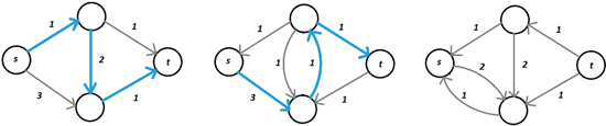
**Figure 6.1:** Augmenting paths in action: At each stage, we route 1 unit of flow along the augmenting path indicated in blue. Observe that at the end there exist no more augmenting paths, so we have found the maximum flow.

6.2 The Max-Flow Min-Cut Duality

To analyze the Augmenting Path Algorithm, we need to introduce some additional definitions.

Definition 6.2. An $(s, t)$ -cut of a capacitated graph $G = (V, c)$ is a partition of $V$ into two sets $(S, T)$ such that $s \in S$ and $t \in T$ . The capacity of an $(s, t)$ -cut $(S, T)$ is the sum of the capacities of all the edges $e = (u, v) \in E_{c}$ such that $u \in S$ and $v \in T$ (i.e., all edges leaving $S$ ). An $(s, t)$ -cut $(S, T)$ is said to be a min- $(s, t)$ -cut in $G$ if its capacity is smaller than, or equal to, the capacity of any other $(s, t)$ -cut in $G$ .

Given an $(s, t)$ -flow $f$ and an $(s, t)$ -cut $(S, T)$ , let $f (S)$ denote the “net flow” from $S$ to $T$ ; that is, $f (S) = \sum_{u \in S, v \in T} f (u, v)$ . Since $(S, T)$ is an $(s, t)$ -cut, any flow traveling from $s$ to $t$ must pass through the edges leaving $S$ , and thus $f (S)$ ought to equal $v a l_{f}$ . This is formalized in the next lemma.

Lemma 6.1. Let $G = (V, c)$ be a capacitated graph, $(s, t)$ a source-sink pair, $f$ an $(s, t)$ -flow for $G$ , and $(S, T)$ an $(s, t)$ -cut of $G$ . Then $v a l_{f} = f (S)$ .

Proof. Recall that

v a l_{f} = \sum_{v | (s, v) \in E_{c}} f (s, v) = \sum_{v \in V} f (s, v) = \sum_{u \in S, v \in V} f (u, v)

where the second equality follows from the fact that $s$ is a source, and the third equality follows from the fact that by the flow conservation condition, for every “internal” node $u \in S ∖ {s}$ , $\sum_{v \in V} f (u, v) = 0$ . Since $(S, T)$ is a partition of $V$ , we can further decompose $\sum_{u \in S, v \in V} f (u, v)$ as:

\sum_{u \in S, v \in S} f (u, v) + \sum_{u \in S, v \in T} f (u, v) .

By the flow symmetry condition, the first term is 0 (since if $f (u, v)$ is in the sum, then so is $f (v, u) = - f (u, v)$ ), and, by definition, the second term is $f (S)$ ; thus, we conclude that $v a l_{f} = f (S)$ .

■

Note that by definition, $f (S)$ is at most the capacity of the cut $(S, T)$ . As a consequence, we directly get the following useful corollary.

Corollary 6.1. Let $G = (V, c)$ be a capacitated graph, $(s, t)$ a source-sink pair, $f$ an $(s, t)$ -flow for $G$ , and $(S, T)$ an $(s, t)$ -cut of $G$ . Then $v a l_{f}$ is at most the capacity of $(S, T)$ .

We are now ready to analyze the Augmenting Path Algorithm.

Theorem 6.1. Given a capacitated graph $G = (V, c)$ and a source-sink pair $(s, t)$ , the Augmenting Path Algorithm outputs some max- $(s, t)$ -flow $f$ in $G$ . Furthermore:

$f$ is always integral;
The algorithm’s running time is polynomial in $| G | \cdot v a l_{f}$ ;
$v a l_{f}$ equals the capacity of any min- $(s, t)$ -cut in $G$ .

Proof. We start by observing that by Claim 6.1 and by an induction over the number of iterations of the algorithm, $f$ remains a valid flow for $G$ throughout the execution of the algorithm. Furthermore, since we are assuming capacities are integers, the extra $Δ$ flow “pushed” along any augmenting path must be an integer, and consequently the residual graph will always have integral capacities. It follows (again by induction) that the flow $f$ remains integral throughout the execution of the algorithm. Additionally, every time we increase the flow along an augmenting path $P$ by $Δ$ , the value of the flow $f$ increases by $Δ$ ; since $Δ > 0$ is an integer, the value of the flow must increase by at least 1 at each iteration. It follows that the number of iterations is bounded by the value, $v a l$ , of the max $(s, t)$ -flow. Moreover, by using BFS and Theorem 2.1, each iteration of the algorithm can be performed in polynomial time in $| G |$ ; thus, we conclude that the overall running time of the algorithm is polynomial in $| G | \cdot v a l$ .

We now show that the final flow is a maximum flow and along the way also prove bullet 3 of Theorem 6.1. By Corollary 6.1, the value of the max- $(s, t)$ flow must be less than or equal to the capacity of every $(s, t)$ -cut in $G$ . Hence, if we show that the flow from $s$ to $t$ at the end of the execution is equal to the capacity of some $(s, t)$ -cut, we have also shown that the flow is maximal; furthermore, this also shows that the value of a max flow equals the capacity of some (and thus any) min cut.

Recall that the algorithm ends when there are no more augmenting paths from $s$ to $t$ . Consider the final residual graph $G_{f}$ at this point. Let $S$ denote the set of nodes that are reachable from $s$ in the directed graph induced by $G_{f}$ (i.e., through edges with positive capacities). Let $T$ be the remaining nodes.

Clearly, $s \in S$ ; because $t$ is unreachable from $s$ (or else the algorithm would not have ended, since there exists an augmenting path from $s$ to $t$ ), $t \in T$ . Thus $(S, T)$ is an $(s, t)$ -cut.
All outgoing edges from $S$ (to $T$ ) must have residual capacity 0 (or else more nodes can be reached from $S$ , and thus $S$ is not the set of nodes that are reachable from $s$ ). Hence, the amount of flow we have routed through those edges must be equal to the capacity of those edges in the original graph $G$ (or else there would be capacity left in the residual graph).
Finally, observe that there cannot be any positive flow on incoming edges to $S$ (from $T$ ), since, if there were some positive flow on an edge $(v, u)$ where $v \in T, u \in S$ , then $f (u, v) < 0$ (by flow symmetry) and thus $c_{f} (u, v) > 0$ , which contradicts the fact that the residual capacity on all outgoing edges is 0.

We conclude that the value of the final flow equals the capacity of the $(s, t)$ -cut $(S, T)$ , which concludes the proof.

■

We mention that special instantiations of the Augmenting Path Algorithm (where we are more careful about which augmenting path $P$ the algorithm selects in each iteration) have an even faster running time for large capacities [EK72], but this will not be of importance to us in this course.

6.3 Bipartite Graphs and Maximum Matchings

Let us now turn to a seemingly different problem (which will turn out to be closely related to the max flow problem): that of finding matchings in bipartite graphs. A bipartite graph is simply a graph where the nodes are divided into two groups—“left nodes” $X$ and “right nodes” $Y$ and edges can only exist between a node in one group and a node in the other. See Figure 6.2 for an example; here the left nodes correspond to a set of professors, the right nodes corresponds to a set of classrooms, and we draw an edge between a professor and the classroom if the classroom is acceptable to the professor.

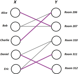
**Figure 6.2:** The edges in purple constitute a maximum matching (of size 4) between professors and classrooms in the bipartite graph.

We here focus only on undirected bipartite graphs:

Definition 6.3. An undirected bipartite graph is an undirected graph $G = (V, E)$ where $V = X \cup Y$ and $E \subseteq {{x, y} | x \in X, y \in Y}$ .

A particular type of bipartite graph of interest is one where the edge set is the full set of edges $E = {{x, y} | x \in X, y \in Y}$ ; we refer to such a graph as a complete bipartite graph over $X \cup Y$ .

Let us turn to defining the notion of a matching; we provide a general definition that applies to all graphs (and not just bipartite ones), but we shall here focus mostly on bipartite graphs.

Definition 6.4. A matching in an undirected graph $G = (V, E)$ is a set of edges $M \subseteq E$ such that every node $v \in V$ has at most degree 1 with respect to $M$ (i.e., at most 1 edge in $M$ connected to it). We define the size of the matching as $|M|$ . We say $M$ is a maximum matching in $G$ if its size is at least as large as the size of any other matching $M^{'}$ in $G$ .

An example of a matching in a bipartite graph can be found in Figure 6.2. An equivalent way to define a matching in an undirected graph $(V, E)$ is as a function $M : V \to V \cup {⊥}$ such that $M (u)$ defines the node $v$ that $u$ gets matched to, or $⊥$ (where $⊥$ denotes an “error” symbol) if $u$ is “unmatched.” More precisely, $M : V \to V \cup {⊥}$ is a function such that (1) for any $u, v \in V$ , if $M (u) = v$ then ${u, v} \in E$ and $M (v) = u$ , and (2) for any $v \in V$ , there exists at most one $u \in V$ such that $M (u) = v$ . To simplify our presentation, we abuse of notation and use both of these formulations/notations of matchings interchangeably.

We now show how to use the Augmenting Path Algorithm to efficiently find maximum matchings in bipartite graphs.

Theorem 6.2. There exists an efficient algorithm that finds the maximum matching in any undirected bipartite graph $G$ in polynomial time in $| G |$ .

Proof. Given an undirected bipartite graph $G = (X \cup Y, E)$ , create an expanded capacitated graph $G^{'}$ with two extra nodes $s$ and $t$ such (a) that the capacity between $s$ and every node in $X$ is 1, (b) the capacity between every node in $Y$ and $t$ is 1, and (c) the capacities along edges $(x, y) \in E$ are set to $| G |$ .¹ (See Figure 6.3 for an illustration.) Note that if $G$ has a matching of size $k$ , then there exists an $(s, t)$ -flow in $G^{'}$ with value $k$ —simply push a flow of 1 from $s$ to every node $u \in X$ that gets matched, and next from $u$ to $u$ ’s match, $v$ , and finally from $v$ to $t$ . In other words, the size of the maximum matching in $G$ is at most the max $(s, t)$ -flow in $G^{'}$ .

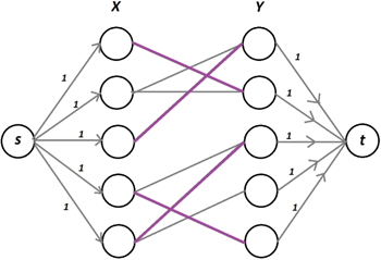
**Figure 6.3:** The graph from Figure 6.2, expanded to create an $s$ - $t$ flow network. The purple edges form a maximum matching.

Now, consider the following algorithm: find the maximum $(s, t)$ -flow $f$ in $G^{'}$ using the Augmenting Path Algorithm, and finally output the edges between $X$ and $Y$ which have flow on them. Since the capacities of the edges connecting $s$ and $t$ to the bipartite graph are 1 (and since there are no edges connecting two nodes in $X$ or two nodes in $Y$ ), by the capacity and conservation of flow constraints, at most 1 unit of flow can pass through each node in $X$ and $Y$ . By Theorem 6.1, the output max flow is integral; hence, the algorithm always outputs a valid matching. Additionally, it follows that the size of the matching is the value of the max flow in $G^{'}$ , and consequently, the matching is of maximum size (since, as argued above, the size of the maximum matching is at most the value of the max flow).

■

6.4 Perfect Matchings and Constricted Sets

Consider now a bipartite graph $G = (X \cup Y, E)$ where $|X| = |Y| = n$ . We are interested in understanding when such a bipartite graph has a perfect matching, where every node gets matched.

Definition 6.5. A matching $M$ in a bipartite graph $G = (X \cup Y, E)$ where $| X | = | Y | = n$ is said to be perfect if all nodes in $X$ get matched in $M$ —that is, $M$ is of size $n$ .

For instance, if $X$ is a set of $n$ men and $Y$ a set of $n$ women, and the edges $(x, y)$ exist between a man-woman pair if they would find a marriage acceptable; a perfect matching exists if and only if everyone can get “acceptably” married.

Note that we can use the above-described maximum matching algorithm to determine when a perfect matching exists. But if the algorithm notifies us that the maximum matching has size $< n$ , it gives us little insight into why a perfect matching is not possible.

Constricted sets The notion of a constricted set turns out to be crucial for characterizing the existence of perfect matchings. Given a graph $G = (V, E)$ , let $N (S)$ denote the set of neighboring nodes to any node in $S$ (that is, $x \in N (S)$ if and only if there exists some $y \in S$ and an edge $(y, x) \in E$ .) A constricted set is a set $C$ of nodes that has less neighbors than elements in $C$ :

Definition 6.6. Given a bipartite graph $G = (X \cup Y, E)$ , a constricted set is a subset $C \subseteq X$ such that $| N (C) | < | C |$ .

Clearly, if a constricted set exists, no perfect matching can be found—a set of $k$ men cannot have acceptable marriages with $< k$ women. The “marriage theorem” proves also the other direction; a perfect matching exists if and only if no constricted set exists. We will show not only this theorem but also how to efficiently find the constricted set when it exists.

Theorem 6.3. Given a bipartite graph $G = (X \cup Y, E)$ such that $| X | = | Y | = n$ , a perfect matching exists in $G$ if and only if no constricted set exists in $G$ . Additionally, whenever such a constricted set exists, it can be found in polynomial time in $| G |$ .

Proof. As already noted above, if there exists a constricted set, then clearly no perfect matching exists. For the other direction, consider a bipartite graph $G = (X \cup Y, E)$ without a perfect matching. We shall show how to efficiently find a constricted set in this graph, which concludes the proof of the theorem.

Consider the expanded capacitated graph $G^{'}$ from the proof of Theorem 6.2; use the max-flow algorithm from Theorem 6.1 to find the max- $(s, t)$ -flow, and consider the min- $(s, t)$ -cut, $(S, T)$ , induced by this flow in the proof of Theorem 6.1. Recall that the set $S$ was obtained by considering the set of nodes that are reachable from $s$ in the final residual graph; this set of nodes can be found in polynomial time using breadth-first search (see Theorem 2.2).

We now claim that $C = S \cap X$ is a constricted set.

Since $G$ does not have a perfect matching, by the proof Theorem 6.2, the max $(s, t)$ -flow in $G^{'}$ is strictly smaller than $n$ . Consequently, by the max-flow/min-cut correspondence of Theorem 6.1, the capacity of the min cut is strictly less than $n$ . Since the outgoing edges from $X$ to $Y$ have capacity $| G | > n$ , none of those edges can connect $S$ to $T$ (otherwise the cut would have capacity at least $n$ , which would be a contradiction).

Thus, the capacity of the min cut is the sum of the number of edges from $s$ to $X \cap T$ and the number of edges from $Y \cap S$ to $t$ ; see Figure 6.4 for an illustration. In other words, the capacity of the min cut is

| X \cap T | + | Y \cap S | < n,

where the inequality follows since, as argued above, the min cut is strictly smaller than $n$ .

On the other hand, since $(S, T)$ is a partition of $X \cup Y$ , it is also a partition of $X$ . Thus,

| X \cap T | + | X \cap S | = n .

Combining the above two equations, we get

| X \cap S | > | Y \cap S | .

Finally, note that since (as argued above) the $(S, T)$ -cut does not cut any edges between $X$ and $Y$ (recall that they have capacities $| G | > n$ ), we have that $N (X \cap S) \subseteq Y \cap S$ . We conclude that

| X \cap S | > | Y \cap S | \geq | N (X \cap S) | .

This proves that $C = X \cap S$ is a constricted set.

■

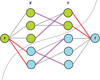
**Figure 6.4:** An illustration of the construction of a constricted set. Edges in the maximum (not perfect) matching are purple; nodes in $S$ are green, nodes in $T$ are blue, and edges leaving $S$ in the min cut are red. Observe that $C = X \cap S$ , the set of green nodes on the left side, forms a constricted set.

Notes

We refer the reader to [CLRS09] and [KT05] for a more in-depth study of graph algorithms. The Augmenting Path Algorithm is due to Ford and Fulkerson [FF62]. The “marriage theorem” is due to Hall [Hal35].

¹For this proof, we can set the capacities along edges in $E$ to any value $\geq 1$ , but for our later usage of this construction it will be useful that the capacities are sufficiently large.