Chapter 19 Markets with Network Effects

Recall our model of networked coordination games (from chapter 4), where the utility of a player’s action depended on (a) the “intrinsic value” of the action to the player, and (b) the coordination (“network”) value of the action, which was a function of the number of its neighbors choosing it.

In this chapter, we will now study markets in a similar setting. Whereas we previously studied markets in a setting where the number of goods for sale was limited (i.e., matching markets), we here consider a market where we have an unlimited number of copies of the good for sale, but buyers still are only interested in buying one item. As we shall see, reasoning about players’ beliefs (and even their higher-level beliefs) will be instrumental for analyzing such scenarios.

19.1 Simple Networked Markets

Concretely, let us consider a scenario where a good can be mass produced at some cost $p$ , and assume that the good is being offered for sale at the same price $p$ ; this models the idea that if there are multiple producers, competition among them will drive the price of the good down to $p + 𝜖$ for some small $𝜖$ .¹

A market without network effects First, consider a simple market with just an intrinsic value for the good, but assume players have different intrinsic values—formally, these values are modeled as player types. Let us, further, assume we have a large set of buyers—let $F (p)$ denote the fraction of the buyers whose intrinsic value $t$ for the good is at least $p$ . As we did in chapter 10, let us consider a quasi-linear utility model, where a buyer’s utility for buying an item is their value for the item minus the price they pay for it. In such a utility mode, a buyer with type $t$ who is rational will only be willing to buy the good if its price $p$ is at most their type, $t$ . Thus, if the good is priced at $p^{*}$ , then assuming all buyers are rational, a $F (p^{*})$ fraction of the buyers will buy it.

Modeling network effects Let us now modify the model by introducing network effects. Toward this end, let us define the value of a good to a player with type (i.e., intrinsic value) $t$ as

v = t d (x),

where $d (x) > 0$ is a “multiplier” modeling the strength of the network effect and $x$ is the fraction of the population that buys the good. We here restrict our study to monotonically increasing multipliers $d (x)$ , so that if more users have the good, the good becomes more valuable (to everyone). (We point out that it may also make sense in some situations to consider a “negative network effect” such that the good becomes less valuable when too many players have it—as the famous Yogi Berra quote goes: “Nobody goes there anymore. It’s too crowded.”)

Analyzing markets with network effects: Self-fulfilling beliefs In such a model, what fraction of the buyers will buy a good? To answer this question, we need to consider the beliefs of the players.

If a buyer with type $t$ believes that an $x$ fraction of the population will buy the good, then their believed value for the good is $v = t d (x)$ .
Thus, if the good is priced at $p^{*}$ , a rational buyer, wishing to maximize their expected utility, will only agree to buy the good if $t \geq \frac{p^{*}}{d (x)}$ .
We conclude that if everyone is rational and believes that an $x$ fraction of the population will buy the good, then an $F (\frac{p^{*}}{d (x)})$ fraction of buyers will actually buy.

Of course, beliefs may be incorrect. So, if people initially believe that, say, an $x_{0} = 0$ fraction of the players will buy the good, then $x_{1} = F (\frac{p^{*}}{d (x_{0})})$ will buy it; but, then, given this, $x_{2} = F (\frac{p^{*}}{d (x_{1})})$ should actually buy it, and so on and so forth—in essence, this iteration gives rise to a best-response dynamics for markets with network effects.

Consequently, following the general theme of this course, we are interested in the “fixed-points,” or equilibria, of this system, where buyers’ beliefs are correct: That is, situations where if everyone is rational and believes that an $x^{*}$ fraction will buy the good, then an $x^{*}$ fraction will actually buy it; we refer to these as self-fulfilling beliefs. More precisely, we refer to a belief $x^{*}$ as a self-fulfilling (with respect to, $F, p^{*}$ ) if

F (\frac{p^{*}}{d (x^{*})}) = x^{*} .

We will also call such an $x^{*}$ an equilibrium.

Stable and unstable equilibria To better understand the structure of self-fulfilling beliefs, let us consider an example. Assume $F (p) = max (1 - p, 0)$ . (So nobody has intrinsic value higher than 1, but everyone has a non-negative intrinsic value.) Let $d (x) = a + b x$ ; we will focus on situations where $a$ is small (so that the value of the good is tiny if nobody else has it) but $b$ is large (so that the value is heavily dependent on the network effect). Self-fulfilling beliefs are characterized by the equation,

x = F (\frac{p^{*}}{d (x)}) = max (1 - \frac{p^{*}}{a + b x}, 0) .

So, $x = 0$ is a self-fulfilling belief if and only if $1 - \frac{p^{*}}{a} \leq 0$ ; that is, when $p^{*} \geq a$ . For any other self-fulfilling belief $0 < x \leq 1$ , it must hold that:

1 - \frac{p^{*}}{a + b x} = x,

which simplifies to:

a + b x - p^{*} = a x + b x^{2}

x^{2} + \frac{a - b}{b} x + \frac{p^{*} - a}{b} = 0 .

By solving the quadratic equation, we get the solutions:

x = \frac{b - a}{2 b} \pm \sqrt{\frac{a - p^{*}}{b} + {(\frac{a - b}{2 b})}^{2}} .

Thus, as we see, there can be between 0 and 3 equilibria, depending on our choice of $a$ , $b$ , and $p^{*}$ . For instance, setting $a = 0.1$ , $b = 1$ , $p^{*} = 0.2$ produces the example shown in Figure 19.1. $x_{0}^{*} = 0$ is a self-fulfilling belief, since $p^{*} > a$ (if everybody believes that nobody will buy the good, the value of the good becomes too low for all the players and thus nobody will want to buy it). The other two equilibria are given by the solutions to the quadratic equation: $x_{1}^{*} \approx 0.13$ and $x_{2}^{*} \approx 0.77$ .

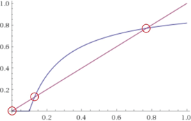
**Figure 19.1:** The function $y = F (\frac{p^{*}}{d (x)})$ for $(a, b, p^{*}) = (0.1, 1, 0.2)$ is plotted in blue, and the function $y = x$ is plotted in red. Equilibria (with respect to $F, p^{*}$ ) are thus characterized by the intersections between plots. Also, notice that BRD will converge to a higher value when $F (\frac{p^{*}}{d (x)}) > x_{1}^{*}$ and lower when $F (\frac{p^{*}}{d (x)}) < x_{1}^{*}$ , which shows that $x_{1}^{*}$ is an unstable equilibrium.

Notice that these three outcomes are actually very different. Which of them will we arrive at assuming that people follow the best-response dynamics considered above? Clearly, if we start at an equilibrium, the BRD process will not move away from it. But what if players’ beliefs are just a touch off (i.e., we start the BRD at a point close to the equilibrium)—will we always converge to the equilibrium point? The answer turns out to be no: In fact, if we start anywhere between $x_{0}^{*}$ and $x_{1}^{*}$ , BRD will converge to $x_{0}^{*}$ , no matter how close to $x_{1}^{*}$ we start! Similarly, if we start at any point greater than $x_{1}^{*}$ , no matter how close to $x_{1}^{*}$ , BRD will converge to $x_{2}^{*}$ . We thus call $x_{0}^{*}$ and $x_{2}^{*}$ stable equilibria; $x_{1}^{*}$ , on the other hand, is an unstable equilibrium.

Tipping points Notice, however, that the equilibrium point $x_{1}^{*}$ is still interesting as a, so-called, tipping point: If everyone believes that more than an $x_{1}^{*}$ fraction of the players will buy the good, we end up at the “good” equilibrium $x_{2}^{*}$ where almost everyone buys it; if people believe that fewer than an $x_{1}^{*}$ fraction of the players will buy the good, we in turn end up at the “bad” equilibrium $x_{0}^{*}$ where nobody buys it!

So, in order to be successful at selling their good, the seller needs to make sure that they achieve a penetration rate of at least $x_{1}^{*}$ . In order to succeed at this, they can lower the price $p^{*}$ of the good to make the “tipping point” lower still. If they lower $p^{*}$ to 0.15, for instance, $x_{1}^{*} \approx 0.06$ ; at 0.11, $x_{1}^{*} \approx 0.01$ ! Thus, to successfully market their good, a seller should be willing to lower the price of their good even below its production cost until they achieve some appropriate penetration rate (above the corresponding “tipping point” to its actual production cost). At that point, they can then safely increase the price back to their production cost.

19.2 Markets with Asymmetric Information

Self-fulfilling beliefs are also a useful tool to analyze markets with asymmetric information—that is, markets where the seller might have more information about the good than the buyers.

The market for lemons Consider a simple market for used cars. We have a large set of cars owned by some sellers:

A fraction $f$ of these cars are “good,” worth $v_{B}$ to buyers but $v_{S} < v_{B}$ to the sellers (note that we assume that all buyers and sellers have the same valuation for a good car).
The remaining cars are “lemons,” worthless to both buyers and the sellers alike.

Sellers may decide to keep their car, or decide to put it up for sale (i.e., placing their car on the market).

How much would a buyer be willing to pay for a random car on the market (i.e., a random car that has been put up for sale), assuming that lemons and good cars are difficult to distinguish. If using the quasi-linear utility model, a rational buyer wishing to maximize their expected utility will only be willing to pay at most

v_{B} x

if they believe that an $x$ fraction of the cars on the market are good.

So, what should a seller do?

If the seller has a lemon, they should clearly put it up for sale, since they might be able to get some money for it.

On the other hand, when the seller has a good car and believes that buyers believe that an $x$ fraction of the cars on the market are good, then if $v_{B} x \geq v_{S},$
they would be willing to put it up for sale, and otherwise they would not (since they will never be able to get more than $v_{S}$ , so no point putting it up for sale).

In fact, to make this last argument, we additionally must assume that common knowledge of rationality holds so that we assume that the seller is rational and believes that all buyers are rational (and thus only buy for at most $v_{B} x$ ).

Analyzing self-fulfilling beliefs: Market crashes To analyze what happens in such a market, we will again consider self-fulfilling beliefs: We say that the belief $x^{*}$ is self-fulfilling (with respect to $v_{s}, v_{b})$ if common knowledge of rationality and common knowledge that “a fraction $x^{*}$ of the cars on the market are good” implies that an $x^{*}$ fraction of the cars on the market actually will be good.

Note that common knowledge of “a fraction $x^{*}$ of the cars on the market are good” means that sellers believe buyers believe an $x^{*}$ fraction of the cars on the market are good. Thus, all sellers believe that all buyers will agree to buy cars for $v_{B} x^{*}$ (but no less). Since all sellers have the same valuation $v_{S}$ for their car, either all of them will put it up for sale, or none. Thus, the only possible self-fulfilling equilibria are:

$x^{*} = f$ (when all sellers put their car up for sale); or,
$x^{*} = 0$ (when no sellers of good cars put them put it up for sale).

The “good” equilibrium when all sellers put their car up for sale can only happen when $v_{S} \leq v_{B} f$ ; that is, when the total fraction $f$ of good cars is at least $\frac{v_{S}}{v_{B}}$ . On the other hand, when $f < \frac{v_{S}}{v_{B}}$ , then the only self-fulfilling equilibrium is $x^{*} = 0$ , where nobody puts good cars up for sale—we get a “market crash” where only sellers with lemons put them up for sale, and nobody is willing to buy!

In fact, the situation is even worse: Even if the original fraction of good cars is high (i.e., $f > \frac{v_{S}}{v_{B}}$ ), if buyers believe that an $x < \frac{v_{S}}{v_{B}}$ fraction of cars on the market are good, then none of them will be willing to buy; as a consequence, sellers of good cars will no longer be willing to sell. In other words, running a best-response dynamics (as above) starting off at some $x < \frac{v_{S}}{v_{B}}$ will lead to the “bad” equilibrium $x^{*} = 0$ (in just one step of the dynamics). On the other hand, if we start off at some $x > \frac{v_{S}}{v_{B}}$ we instead converge to $x^{*} = \frac{v_{S}}{v_{B}}$ (again, in just one step).

We conclude that $t = \frac{v_{S}}{v_{B}}$ is the “tipping point” for the market: if the sellers believe that the buyers believe that the fraction of good cars on the market is smaller than $\frac{v_{S}}{v_{B}}$ , they will not be willing to sell good cars, and the market crashes (as before, only lemons are put on the market, and nobody will be willing to buy them).

Of course, it is unrealistic to assume that every good car has the same value. But even if there are several different types of cars (e.g., “excellent,” “very good,” “good,” “bad,” and “lemons”), but different quality cars are indistinguishable to buyers, if buyers’ beliefs on the “quality of the market” fall below some appropriately defined tipping point, none of the “excellent” cars will enter the market, which will drive down the expected value of a random car and consequently drive out all the “very good” ones, which will drive out the “good” ones, and so on, until only lemons remain in the market! So we get the same type of market crash also in more realistic models. (Indeed, 5 years after Akerlof’s seminal paper on markets for lemons [Ake95] was published, the United States enacted federal “lemon laws” to protect buyers against purchases of lemons.)

Extension to labor markets Finally, let us mention that this sort of market crash occurs not only in used car sales but also in, for instance, labor markets where an employer might not be able to effectively evaluate the skills of a worker. Consider, for instance, a simple setting where we have two types of workers (“good workers” and “bad workers”): Good workers are analogous to the good cars, and have some value $v_{S}$ they can generate on their own (e.g., being self-employed) and some other value $v_{B}$ they can contribute to the employer; bad workers are the “lemons” of the market (worth nothing on their own and to the employer). The exact same analysis as above applies to this situation assuming the employer cannot distinguish the two types of worker.

Spence’s signaling model (Or: why university degrees are useful, even if you don’t actually learn anything!) One way around this problem is to let players signal the value of their good. For the labor market, education can be used as such a signal. Assume that getting a university degree is more costly for a bad worker than for a good one (due to, say, fewer scholarships, more time required, etc.). If companies set different base salaries depending on whether the worker has a degree or not, they may end up at a “truthful equilibrium” where bad workers do not get degrees because the added salary is not worth the extra cost of the degree to them, while for good workers, getting the degree will be worthwhile, since the extra salary outweighs the (lower) cost of the education. So, getting a degree may be worthwhile to the good workers—even if they do not gain any relevant skills or knowledge—as their willingness to get the degree signals their “higher value” as an employee.

Notes

Our treatment of markets with network effects follows models from [KS85, SV13] (see also the treatment in [EK10]). Markets for lemons were first explored in the work of Akerlof [Ake95], and “Spence’s signaling model” in the work of Spence [Spe73]. Michael Spence, George Akerlof, and Joseph Stiglitz shared the 2001 Nobel Prize in Economic Sciences for their work on markets with asymmetric information.

¹At this point, the astute reader may ask: why would anyone ever want to produce a good if they only recover their production cost? The point is that the production cost here includes also the “cost of financing”—for example, whatever revenue shareholders of the company producing the good are expecting to get.