Chapter 12 Voting: Barriers and Ways around Them

In this chapter, we continue our exploration of voting: we present a fundamental barrier to strategy-proof voting (the Gibbard–Satterthwaite theorem), and next exemplify some ways to circumvent this barrier.

12.1 The Gibbard–Satterthwaite Theorem

Roughly speaking, the Gibbard-Satterthwaite theorem shows that if we restrict to voting rules that are onto—where all candidates can win—then the only strategy-proof voting rule over three or more candidates is “dictatorship.”

We start by formalizing what it means for a voting rule to be onto (i.e., that it is feasible for every candidate to be able to win):

Definition 12.1. Given a complete social-choice context $Γ = (n, Ω, T, v)$ , we say a voting rule $𝒱$ is onto if for every candidate $x \in Ω$ , there exists some preference profile $\vec{μ} \in T$ such that $𝒱 (\vec{μ}) = x$ .

Let us turn to defining what it means for a voting rule to be dictatorial.

Definition 12.2. Given a complete social-choice context $Γ = (n, Ω, T, v)$ , we say that a voter $i$ is a dictator for $x$ with respect to $𝒱$ if $𝒱 (\vec{μ}) = x$ for every $\vec{μ}$ such that $i$ ranks $x$ first. We say that $i$ is simply a dictator for $𝒱$ if for every $x \in Ω$ , $i$ is a dictator for $x$ with respect to $𝒱$ . We finally call a voting rule $𝒱$ dictatorial if there exists some voter $i$ such that $i$ is a dictator for $𝒱$ .

A useful property of the notion of dictatorship is that if a voter $i$ is a dictator for some candidate $a \in Ω$ , then no other voter $i^{'}$ can be a dictator for some other candidate $b \neq a$ (since the situation where $i$ ranks $a$ first and $j$ ranks $b$ first would lead to a conflict).

Note that any dictatorial voting rule $𝒱$ clearly is onto and strategy-proof. The Gibbard–Satterthwaite theorem shows a surprising converse of this observation:

Theorem 12.1 (The Gibbard–Satterthwaite theorem). Let $𝒱$ be a voting rule that is onto and strategy-proof for some complete social-choice context with strict preferences over at least three outcomes. Then $𝒱$ is a dictatorial.

Note that a direct corollary of this theorem is that voting rules for social-choice contexts with strict preferences, in general, we cannot DST-implement social value maximization (since for most social-choice contexts, dictatorship clearly will not implement social value maximization; we leave it as an exercise to prove this).

12.2 Proof of the Gibbard–Satterthwaite Theorem [Advanced]

For simplicity of notation, in the remainder of this section, we always have some fixed complete social-choice context $Γ$ over at least three outcomes and with strict preferences, in mind (and as such, whenever we write strategy-proof, or onto, we mean with respect to this social-choice context). Before turning to the actual proof, let us first demonstrate that strategy-proof voting rules satisfy two natural properties that we would expect from any “reasonable” voting rule.

Definition 12.3. A voting rule $𝒱$ is monotone if for every two preference profiles $\vec{μ}$ and ${\vec{μ}}^{'}$ , if $𝒱 (\vec{μ}) = x$ , and for every player $i$ and every candidate $y$ such that $x >_{μ_{i}} y$ it is also true that $x >_{μ_{i}^{'}} y$ , it follows that $𝒱 ({\vec{μ}}^{'}) = x$ .

In other words, if a voting rule is monotone, then a winning candidate $x$ will continue to win as long as, for any player $i$ , all candidates that are dominated by $x$ continue being dominated by $x$ .

Definition 12.4. A voting rule $𝒱$ is Pareto-optimal if for every profile $\vec{μ}$ and candidate $x$ such that $x >_{μ_{i}} y$ for every player $i$ , we have that $𝒱 (\vec{μ}) \neq y$ .

In other words, if a voting rule is Pareto-optimal, then no candidate $y$ , that is dominated by some candidate $x$ in every player’s preference ordering, can ever win. In particular, if a candidate $x$ is preferred by all players, that candidate must win.

The following two lemmas state that strategy-proof voting rules are both monotone and Pareto-optimal.

Lemma 12.1. Any strategy-proof voting rule $𝒱$ is monotone.

Proof. Assume for contradiction that $𝒱$ is not monotone; then, there exist profiles of preferences $\vec{μ}$ and ${\vec{μ}}^{'}$ so that $𝒱 (\vec{μ}) = x$ and for every player $i$ and every candidate $y$ such that $x >_{μ_{i}} y$ it is also true that $x >_{μ_{i}^{'}} y$ , and yet $𝒱 ({\vec{μ}}^{'}) \neq x$ .

We construct a sequence of “hybrid” preferences ${\vec{μ}}^{k}$ where we move from $\vec{μ}$ to ${\vec{μ}}^{'}$ one player at a time:

$μ_{i}^{k} = μ_{i}$ if $i > k$ , and
$μ_{i}^{k} = μ_{i}^{'}$ if $i \leq k$ .

(See Figure 12.1 for an illustration of the hybrid preference profiles.) Thus, ${\vec{μ}}^{0} = \vec{μ}$ and ${\vec{μ}}^{n} = {\vec{μ}}^{'}$ . Now let $k^{*}$ denote the smallest index where $𝒱 ({\vec{μ}}^{k^{*}}) = x$ but $𝒱 ({\vec{μ}}^{k^{*} + 1}) = z \neq x$ . Clearly such an index must exist, since $𝒱 ({\vec{μ}}^{n}) \neq x$ by assumption.

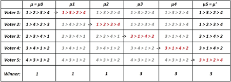
**Figure 12.1:** An example of the hybrid preference profiles in the proof of Lemma 12.1. In this case, we can see that the winner does change between $\vec{μ}$ and ${\vec{μ}}^{'}$ , despite the fact that every player who prefers 1 to any other candidate in $\vec{μ}$ still prefers 1 to the same candidates in ${\vec{μ}}^{'}$ . The example shows that the voting rule (here, plurality with ties broken by largest candidate number) is not monotone and hence not strategy-proof.

Furthermore, note that the only difference between ${\vec{μ}}^{k^{*}}$ and ${\vec{μ}}^{k^{*} + 1}$ is that player $k^{*} + 1$ is switching from $μ_{k^{*} + 1}$ to $μ_{k^{*} + 1}^{'}$ . Since $𝒱$ is strategy-proof, we must have that $x >_{μ_{k^{*} + 1}} z$ , or else, given the preference profile ${\vec{μ}}^{k *}$ , player $k^{*} + 1$ would prefer to report $μ_{k^{*} + 1}^{'}$ , which would lead to the outcome $z$ that they strictly prefer to $x$ (by our assumption that preferences are strict). Since by the choice of $\vec{μ^{'}}$ , we have that for every player $i$ and every choice $y$ , if $x >_{μ_{i}} y$ then $x >_{μ_{i}^{'}} y^{'}$ , it follows that $x >_{μ_{k^{*} + 1}^{'}} y$ .

But, by the same argument, we have that $z >_{μ_{k^{*} + 1}^{'}} x$ (or else player $k^{*} + 1$ would prefer to report $μ_{k^{*} + 1}$ given the preference profile ${\vec{μ}}^{k * + 1}$ ); this is a contradiction (since preferences are strict).

■

Lemma 12.2. Any strategy-proof and onto voting rule $𝒱$ is Pareto-optimal.

Proof. Assume for the sake of contradiction that there exists some preference profile $\vec{μ}$ and some candidate $x$ such that $x >_{μ_{i}} y$ for every player $i$ , yet $𝒱 (\vec{μ}) = y$ . Now:

Let ${\vec{μ}}^{'}$ be a modified version of $\vec{μ}$ where candidates $x, y$ are “pushed-up” so that $x$ is every player’s first choice and $y$ is every player’s second choice. (For instance, if we have two voters with preferences $a > b > x > c > y$ and $c > x > a > y > b$ in $\vec{μ}$ , respectively, their preferences in ${\vec{μ}}^{'}$ will become $x > y > a > b > c$ and $x > y > c > a > b$ .) By monotonicity, we must still have that $𝒱 ({\vec{μ}}^{'}) = y$ (since all candidates dominated by $y$ still are dominated by it).
Since $𝒱$ is onto, there must exist some preference profile $\vec{ν}$ such that $𝒱 (\vec{ν}) = x$ . Let ${\vec{ν}}^{'}$ be the modified version of $\vec{ν}$ where $x$ and $y$ are “pushed-up” in the same way as before. Again, by monotonicity, we have $𝒱 ({\vec{ν}}^{'}) = x$ .
Finally, by monotonicity applied to the transition from ${\vec{ν}}^{'}$ to ${\vec{μ}}^{'}$ , it follows that $𝒱 ({\vec{μ}}^{'}) = x$ , since we are only moving around candidates that are dominated by $x$ (and $y$ )).

The conclusion of bullet 3 (i.e., that $𝒱 ({\vec{μ}}^{'}) = x$ ) contradicts the conclusion of bullet 1 (i.e., that $𝒱 ({\vec{μ}}^{'}) = y$ ), which concludes the proof of the lemma.

■

We are now ready to prove the Gibbard–Satterthwaite theorem.

Proof of the Gibbard–Satterthwaite theorem. First, note that the theorem for the case that $n = 1$ directly follows from Pareto-optimality of $𝒱$ . We next prove the theorem for the case that $n = 2$ , and then proceed to prove the general case by induction.

The special case of 2 voters ( $n = 2$ ) Toward proving the theorem for the special case of 2 votes, let us first prove the following easier claim.

Claim 12.1. Consider some strategy-proof and onto voting rule $𝒱$ for two voters, and any ordered pair of candidates $(a, b)$ where $a, b \in Ω$ . Then, either player 1 is a dictator for $a$ with respect to $𝒱$ , or player 2 is a dictator for $b$ with respect to $𝒱$ .

Proof. Consider any two candidates $a$ and $b$ in $Ω$ . Let profile $μ_{1}$ be some arbitrary ranking where $a$ is first and $b$ is second, and let $μ_{2}$ be the same ranking except that we switch the order of $a$ and $b$ . (For instance, if we let $μ_{1}$ be $a > b > x > y > z$ , then $μ_{2}$ becomes $b > a > x > y > z$ .) Note that by Pareto-optimality either $a$ or $b$ must win the election (i.e., $𝒱 (\vec{μ}) \in {a, b}$ ), since all other candidates are dominated by both $a$ and $b$ for both players. Let us first consider the case that $a$ wins (i.e., $𝒱 (\vec{μ}) = a$ ).

Now consider a new profile of rankings $(μ_{1}, μ_{2}^{'})$ where $μ_{2}^{'}$ is identical to $μ_{2}$ except $a$ is ranked last for player 2. (For instance, in the example above, $μ_{2}^{'}$ becomes $b > x > y > z > a$ .)

By Pareto-optimality, we still have that either $a$ or $b$ must win, since all other candidates are still dominated by $b$ .
However, by strategy-proofness, $b$ cannot win now, since in this case player 2 would have preferred to report $μ_{2}^{'}$ in the original profile $\vec{μ}$ (where $a$ wins but player 2 prefers $b$ ).
So, $a$ must still be winning with respect to the new profile $(μ_{1}, μ_{2}^{'})$ .
By monotonicity (transitioning from $(μ_{1}, μ_{2}^{'})$ to ${\vec{μ}}^{″}$ ) it follows that $𝒱 ({\vec{μ}}^{″}) = a$ for every profile of rankings ${\vec{μ}}^{″}$ where player 1 ranks $a$ on top, since in any such ranking $a$ still dominates all other candidates for player 1 (and monotonicity holds vacuously for player 2, since $a$ dominates no other candidate in $μ_{2}^{'}$ ).

Thus, we conclude that player 1 is a dictator for $a$ with respect to $𝒱$ . Symmetrically, in the case that $𝒱 (\vec{μ}) = b$ , player 2 is a dictator for $b$ .

■

Now we can apply this claim to three candidates.

Claim 12.2. Consider some strategy-proof and onto voting rule $𝒱$ for two voters. Given any set of candidates $a, b, c \in Ω$ , we have that either player 1 or player 2 is a dictator for all three candidates with respect to $𝒱$ .

Proof. We simply apply Claim 12.1 to different subsets of the three candidates:

Applying Claim 12.1 to the pair

(a, b)

, we get that either 1 is a dictator for

a

or 2 is a dictator for

b

. Assume, for now, that the first case holds (i.e., 1 is a dictator for

a

Next, applying Claim 12.1 to the pair $(b, c)$ , we get that either 1 is a dictator for $b$ or 2 is a dictator for $c$ . But since we already assumed that 1 is a dictator for $a$ , 2 cannot be a dictator for $c$ (or else we would get a conflict in the definition of $𝒱$ , as noted above). Hence, 1 must be a dictator for both $a$ and $b$ .

Finally, applying Claim 12.1 to the pair

(c, a)

, we get that either 1 is a dictator for

c

or 2 is a dictator for

a

. Again, 2 cannot be dictator for

a

since we have shown that 1 is a dictator

b

; thus, 1 must also be a dictator for

c

We thus conclude that 1 is a dictator for all three candidates. By symmetry, if the second case held initially (i.e., player 2 was a dictator for

b

), player 2 would become a dictator for all candidates.

This concludes the proof of the claim.

■

We can finally conclude the proof of the theorem for the case that $n = 2$ by applying Claim 12.2 to all triples $(a, b, x)$ , $x \neq a, b$ , and again observing that since 1 and 2 cannot simultaneously be dictators for both $a$ and $b$ , one of the players must be a dictator for every candidate.

The general case ( $n \geq 2$ ) Next, to prove the theorem for any number of voters, we proceed by induction. The base case ( $n = 2$ ) has already been proven above. For the induction step, assume that the theorem is true for $n - 1$ voters; we shall prove it holds for $n$ voters. Assume for contradiction that this is not the case. That is, there exists some onto and strategy-proof voting rule $𝒱$ with $n$ voters that is not dictatorial.

Let $μ^{x}$ be a preference ordering where $x$ is ranked highest and all other candidates are ranked according to a lexicographic order, and define an $(n - 1)$ -player voting rule, $𝒱^{x}$ which simply runs $𝒱$ but fixes the first player’s vote to $μ^{x}$ ; that is,

𝒱^{x} (\vec{μ}) = 𝒱 (μ_{x}, \vec{μ}) .

First, note that since $𝒱$ is strategy-proof, we have that for every candidate $x \in Ω$ , $𝒱^{x}$ is strategy-proof. Next, as we show below, $𝒱^{x}$ also is onto. (Looking forward, we will then use the induction hypothesis to conclude that $𝒱^{x}$ —which has $n - 1$ voters—is dictatorial, and then use this fact to conclude that also $𝒱$ must be dictatorial.)

Claim 12.3. For every $x \in Ω$ , we have that $𝒱^{x}$ is onto.

Proof. Toward showing this claim, consider a different voting rule $\tilde{𝒱}$ for just 2 voters:

\tilde{𝒱} (μ_{1}, μ_{2}) = 𝒱 (μ_{1}, μ_{2}, μ_{2}, \dots, μ_{2}) .

(That is, the 2-party voting rule $\tilde{𝒱}$ repeats player 2’s vote $n - 1$ times and next runs $𝒱$ .) Note that $\tilde{𝒱}$ must be onto, since for every $y \in Ω$ ,

\tilde{𝒱} (μ^{y}, μ^{y}) = 𝒱 (μ^{y}, μ^{y}, \dots, μ^{y}) = y

due to the fact that $𝒱$ satisfies Pareto-optimality. Since $𝒱$ is strategy-proof, $\tilde{𝒱}$ must be strategy-proof for player 1; by the following argument, it must also be so for player 2:

Assume for contradiction that $\tilde{𝒱}$ is not strategy-proof for player 2; then there exists $μ_{1}, μ_{2}, μ_{2}^{'}$ such that $\tilde{𝒱} (μ_{1}, μ_{2}^{'}) >_{μ_{2}} \tilde{𝒱} (μ_{1}, μ_{2})$ .
Now, consider $\tilde{𝒱} (μ_{1}, μ_{2}) = 𝒱 (μ_{1}, μ_{2}, μ_{2}, \dots, μ_{2})$ and switch one player at a time from $μ_{2}$ to $μ_{2}^{'}$ until we arrive at $\tilde{𝒱} (μ_{1}, μ_{2}^{'})$ ; let ${\vec{μ}}^{k}$ , where $k \in [n - 1]$ denote the $k^{th}$ such “hybrid” preference profile.
Since $\tilde{𝒱} (μ_{1}, μ_{2}^{'}) = 𝒱 ({\vec{μ}}^{n - 1}) >_{μ_{2}} \tilde{𝒱} (μ_{1}, μ_{2}) = 𝒱 ({\vec{μ}}^{0})$ , there must exist some $k^{*}$ such that $𝒱 ({\vec{μ}}^{k^{*} + 1}) >_{μ_{2}} 𝒱 ({\vec{μ}}^{k^{*}})$
and thus also
$𝒱 ({\vec{μ}}^{k^{*} + 1}) >_{μ_{k^{*}}^{k^{*}}} 𝒱 ({\vec{μ}}^{k^{*}}),$
which contradicts strategy-proofness for player $k^{*}$ with respect to $𝒱$ .

So (by the already proven base case) $\tilde{𝒱}$ must be dictatorial. If player 1 is a dictator for $\tilde{𝒱}$ , then, by monotonicity, it follows that 1 must be a dictator also for $𝒱$ , which is a contradiction (since we assumed that $𝒱$ was not dictatorial). Thus, player 2 must be the dictator for $\tilde{𝒱}$ ; in other words, for every $y \in Ω$ , and every preference ordering $μ$ , it holds that

\tilde{𝒱} (μ, μ^{y}) = y .

In particular, it holds that

𝒱^{x} (μ^{y}, μ^{y}, \dots, μ^{y}) = \tilde{𝒱} (μ^{x}, μ^{y}) = y

so we conclude that $𝒱^{x}$ is onto.

■

Thus, we have shown that for every $x$ , $𝒱^{x}$ is both onto and strategy-proof. By the inductive hypothesis it thus follows that for every $x \in Ω$ , $𝒱^{x}$ (having $n - 1$ participating voters) is dictatorial. This does not directly give us that also $𝒱$ is dictatorial (which would conclude the proof) since apriori, there may exist $x_{1}, x_{2} \in Ω$ , such that $𝒱^{x_{1}}$ has a different dictator (say $i_{1}$ ) than $𝒱^{x_{2}}$ has (say $i_{2}$ ). However, as we now show, if that were to happen, $𝒱$ could not be strategy-proof for player $1$ .

Consider the preference profile $\vec{μ}$ where player $i_{1}$ has preferences $μ^{x_{2}}$ (i.e., ranks $x_{2}$ highest) and all other players have preferences $μ^{x_{1}}$ . If everyone votes truthfully, since player 1’s preferences are $μ^{x_{1}}$ , the outcome will be

𝒱 (\vec{μ}) = 𝒱^{x_{1}} (μ_{- 1}) = x_{2}

since $i_{1}$ is a dictator for $𝒱^{x_{1}}$ , and $i_{1}$ chooses $μ^{x_{2}}$ . If player 1, however, had misreported their preferences and instead reported $μ^{x_{2}}$ , then the outcome would be $𝒱^{x_{2}} (μ_{- 1}) = x_{1}$ since $i_{2}$ is a dictator $𝒱^{x_{2}}$ and $i_{2}$ chooses $μ^{x_{1}}$ . So player 1 prefers to misreport their preferences (reporting $μ^{x_{2}}$ as opposed to $μ^{x_{1}}$ ) and thus $𝒱$ is not strategy-proof, which is a contradiction.

We conclude that there exists a single player $i$ such that for every $x \in Ω$ , player $i$ is a dictator for $𝒱^{x}$ , and thus player $i + 1$ is a dictator also for $𝒱$ ; this concludes the proof.

■

12.3 Single-peaked Preferences and the Median Voter Theorem

The above impossibility result (i.e., the Gibbard–Satterthwaite theorem) relies on the fact that voters’ preferences over candidates can be arbitrary. In other words, it relies on the fact that the social-choice context is complete. Under a natural restriction on the preferences, it can be overcome. In fact, as it turns out, under the same restriction, we can also overcome the impossibility of Condorcet voting.

Roughly speaking, we say that preferences are single-peaked if all candidates can be placed on a one-dimensional spectrum (e.g., think of the American political spectrum in terms of liberal/left and conservative/right), and voters’ valuations for candidates strictly decrease based on how far they are to the left or right of their “ideal outcome” on the spectrum—that is, the valuation decreases with distance to some ideal point, but might decrease differently depending on whether it is to the left or right of that point. See Figure 12.2 for an illustration.

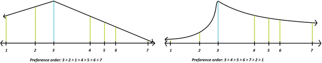
**Figure 12.2:** An illustration of the intuition behind single-peaked preferences. In this example, seven candidates are arranged on a spectrum. We can imagine the voter’s preferences as a function over this spectrum; the only requirements for this function are that it must be maximized at the voter’s top choice (in this case, 3), and strictly decreasing as distance from that choice increases. In the first example (left), the preference diminishes directly with distance; in the second example (right), it does not, which preserves the voter’s top choice but changes the order of preferences. In fact, any preference where $3 > 2 > 1$ and $3 > 4 > 5 > 6 > 7$ is admissible as single-peaked.

More formally, we say that a social-choice context $Γ = (n, Ω, T, v)$ has single-peaked preferences if (a) $Γ$ has strict preferences, and (b) there exists some “global” ordering $x_{1}, x_{2}, \dots, x_{n}$ over the candidates in $Ω$ such that for each player $i$ , the type set $T_{i}$ is the set of preferences $μ$ for which there exists some “ideal candidate” $i^{*}$ such that for all $i < j$ :

if $i^{*} < i < j$ , then $x_{i} >_{μ} x_{j}$ ;
if $i < j < i^{*}$ , then $x_{j} >_{μ} x_{i}$ .

The celebrated median voter theorem by Black [Bla48] shows that once we restrict to social-choice contexts with single-peaked preferences, a Condorcet winner always exists—in fact, the preferred choice of the so-called “median voter” will be a Condorcet winner. We additionally remark that this median-voter mechanism is also strategy-proof:

Theorem 12.2 (The median voter theorem). There exists a strategy-proof voting rule $𝒱$ for all single-peaked social-choice contexts; furthermore, $𝒱$ will always select a Condorcet winner for all single-peaked social-choice contexts.

Proof. For simplicity, let us begin by assuming an odd number of voters. Let $a_{1}, \dots, a_{n}$ denote the top choices of each voter’s reported preferences, ordered according to the one-dimensional spectrum. Let $𝒱$ output $a^{*} = a_{\frac{n + 1}{2}}$ (i.e., the preference of the median voter according to the spectrum). See Figure 12.3 for an example.

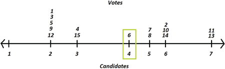
**Figure 12.3:** An example of the median voter rule with 15 voters and the seven candidates from the previous figure. If we order the 15 votes according to their positions on the spectrum, voter 6 is the median (eighth) vote, and so his candidate (4) wins, despite candidate 2 having a plurality of the votes. This rule is strategy-proof assuming single-peaked preferences, but may still leave a lot of voters unhappy and definitely does not maximize social welfare. (*Exercise*: Try to come up with a preference function for each voter to show this.)

$𝒱$ produces a Condorcet winner Consider any alternative candidate $a_{i}$ such that $i < \frac{n + 1}{2}$ (i.e., $a_{i}$ is to the “left” of $a^{*}$ on the spectrum). All $\frac{n + 1}{2}$ voters including, and to the right of, $a^{*}$ must prefer $a^{*}$ to $a_{i}$ , by the single-peaked preferences requirement. Symmetrically, if $a_{i}$ is to the “right” of $a^{*}$ , then all $\frac{n + 1}{2}$ voters including, and to the left of, $a^{*}$ must prefer $a^{*}$ to $a_{i}$ . So at least $n / 2$ voters prefer $a^{*}$ to any other candidate, and so $a^{*}$ is a Condorcet winner.

$𝒱$ is strategy-proof Clearly, the median voter is not incentivized to report his preference falsely, as they are receiving optimal utility (their top choice) by reporting truthfully. Voters to the left of the median cannot change the median by deviating, except by pushing it to the right by voting for a candidate to the right (and thus losing utility by the single-peaked preference rule); symmetrically, voters to the right can only push the median to the left by deviating (and again lose utility). Thus, the voting rule is strategy-proof.

Dealing with even $n$ Now, if $n$ is even, we can just take the median vote to be $a^{*} = a_{n / 2}$ . We still have that $𝒱$ is strategy-proof by the same logic as above. In addition, $𝒱$ will still output a Condorcet winner; $a^{*}$ will be preferred to an alternative candidate to the left by $n / 2 + 1$ voters (all voters including and to the right of $a^{*}$ ), and will be preferred to an alternative candidate to the right by at least $n / 2$ voters (all voters including and to the left of $a^{*}$ ).

■

Notice that in case $n$ is odd, the above proof shows that there is a unique Condorcet winner, whereas when $n$ is even, there can be at most 2 ( $a_{n / 2}$ and $a_{n / 2 + 1}$ ).

12.4 Voting with Payments

Finally, let us revisit the question of designing mechanisms for social-choice contexts, but this time allowing for payments—that is, the mechanism can now charge players based on how they vote. For concreteness, consider again a specific social-choice context with two players (voters) and where the set of outcomes $Ω$ is ${A, B}$ ; recall that a mechanism $ℳ$ for this social-choice context needs to output a winning candidate and prices for the voters to pay. There are just two types of players $t_{1} = (A, B)$ , and $t_{2} = (B, A)$ ; let the valuations for the players be such that player 1 (having type $t_{1}$ ) gets utility 10 if $A$ gets elected, and 0 if $B$ gets elected, whereas player 2 (having type $t_{2}$ ) gets utility $4$ if $A$ gets elected and $6$ if $B$ .¹ (This example is essentially isomorphic to the airport vs. train station example from chapter 10, but using a different type space.)

Consider applying the VCG mechanism (with the Clarke pivot rule) to this context. The outcome maximizing social value is $A$ winning (with a social value of $10 + 4 = 14$ as opposed to $0 + 6 = 6$ for $B$ winning); thus, the VCG mechanism will pick this outcome assuming players truthfully report their types. Now, consider the externality of each player. If player 1 were not voting, $B$ would win and player 2 would receive 6 in utility; however, with player 1 voting and $A$ winning, player 2 only receives 4. Hence, player 1’s externality is 2. Player 2’s externality is 0, since the outcome is the same for player 1 regardless of whether player 2 votes or not. So in this case, player 1 would be charged a price of 2 by the VCG mechanism with the Clarke pivot rule, whereas player 2 would not be charged anything.

One interesting thing to note about this mechanism is that only a “pivotal player” who can actually change the outcome of the election has to pay anything (in the example above, player 1); they, in addition, never need to pay more than their difference in value between the two candidates.

Knowledge of valuations Note that to apply the VCG mechanism to a social-choice context, the mechanism needs to know by how much each player values their respective candidate (i.e., the the mechanism needs to know the utility function)—this is needed since the players’ types (that they report to the mechanism) are simply a ranked list of candidates. It is not clear how the voting authority (running the VCG mechanism) can obtain these valuations in a reliable way.

But there is an easy fix: just as we did in the airport vs. train station example in chapter 10, let us consider a more general mechanism design context for social choice where a player’s type not only specifies a preference order, but also specifies how valuable each candidate is to the player! We can still apply the VCG mechanism to such a context, and the result would be that players now are incentivized to truthfully report exactly how valuable each candidate is to them (and we would still recover the same outcome described above, except that now player 1 would report $(A, 10), (B, 0)$ and player 2 would report $(A, 4), (B, 6)$ ).

So, we have a practical mechanism that enables us to elect a candidate that maximizes social value. Why aren’t all the countries in the world switching to using this VCG mechanism? We highlight a few answers (think about others yourself!):

As already mentioned, in the context of voting, maximizing social value may not be the “right” desiderata: a richer player may have more to gain/lose from the outcome of the election, and such a player’s preferences will receive a heavier weight. This, intuitively, seems unfair and undesirable.
But even if we decide that social value maximization is what we want to achieve, there is a problem with running this mechanism in an uncontrolled environment: collusion. Consider a scenario with 100 voters, 98 of whom prefer $A$ , but the other two of them want to bias the election so that $B$ wins and they do not have to pay anything. Let us say that they both decide to bid an outrageous sum of money (say, 10 billion dollars), equal to far more than the combined sum of the $A$ supporters valuations. Clearly, if either one of them were to not vote, the outcome of the election would be $B$ , so, neither of them has any externality, and they would thus pay nothing! This is an example of how collusion between players breaks the truthfulness of the VCG mechanism. (We mention that the same problem occurs also in the case of auctions, which is why there are regulations against collusion when running, for example, spectral auctions.)

12.5 Summarizing the Voting Landscape

Let us informally summarize the key feasibility and infeasibility results obtained for strategy-proof voting:

For the case of 2 candidates, there exists a strategy-proof voting rule that always selects a Condorcet winner: in fact, the most natural rule—plurality—of selecting the candidate with the most number of top-choice votes works.
For the case of 3 or more candidates, the only strategy-proof voting rule is dictatorship (as shown by the Gibbard–Satterthwaite theorem), and no voting rule can always elect a Condorcet winner.
But with restricted preferences (single-peaked ones, where the candidates can be placed on a one-dimensional spectrum), a natural voting rule (selecting the median voter’s top choice) is both strategy-proof and always selects a Condorcet winner.
Finally, with payments, DST voting maximizing social value is possible (but the mechanism is vulnerable to attacks by collusion between two or more voters).

Notes

The Gibbard–Satterthwaite theorem was first proved in [Gib73, Sat75]; this result is closely related to an earlier impossibility result by Kenneth Arrow [Arr50], demonstrating that a different set of desirable properties for voting rules are inconsistent; Arrow received the Nobel Prize in Economic Sciences in 1972.

Our proof of the Gibbard–Satterthwaite theorem is new but follows high-level ideas from the proofs in [SR14] and [BP90]. Single-peaked preferences and the median voter theorem are due to Black [Bla48].

The Gibbard–Satterthwaite theorem can be extended in various ways. First, the theorem only talks about deterministic voting rules, but as shown by Gibbard [Gib77] it can also be extended to randomized ones. Additionally, the notion of strategy-proofness is quite strong as it requires an implementation in dominant strategies (that is, truthfully reporting your preferences is always a best response, no matter what the other players do). As mentioned in the previous chapters, a weaker form of truthful implementation is that of Bayes–Nash truthful implementation; in the context of voting, the notion of “Bayes–Nash strategy-proofness” would require that truthfully reporting your preferences maximizes expected utility assuming everyone else reports their true preferences, where the expected utility is computed assuming all other players’ types are independently drawn from some distribution $D$ —this distribution $D$ describes how players believe others will vote (e.g., $D$ could be obtained from polling). Unfortunately, as shown by McLennan [McL11], the Gibbard–Satterthwaite theorem actually extends also to this setting! However, as shown in [LLP15], McLennan’s result requires Bayes–Nash strategy-proofness to hold with respect to all distributions $D$ , even those that are very “complicated” in the sense that they require high precision (i.e., a large number of decimal points) to describe the probabilities assigned to various candidates. In contrast, [LLP15] demonstrates natural voting rules that satisfy Bayes–Nash strategy-proofness with respect to distributions $D$ , where only a small number of decimal points are used to describe probabilities (i.e., when players’ beliefs are “coarse” as one would expect them to be).

¹Formally, player 1’s utility function is such that the player gets 10 in utility if their top choice wins (according to the player’s type) and 0 otherwise, whereas player 2’s utility is such that they get 6 if their top choice wins, and 4 otherwise.