BLOKE: Optimizing Bril with STOKE
We present BLOKE, a scalable implementation of STOKE on an educational intermediate representation language. In contrast to STOKE’s two-stage process, BLOKE supports a user-defined number of phases that smoothly transitions from synthesis to optimization. We found that BLOKE was able to find superoptimizations of loop-free code written in Bril. Furthermore, we found BLOKE to be scalable with respect to the number of cores a machine has.
This blog post is a rendition of this report. I also gave a presentation on this project which has palatable slides.
Introduction
Compiler optimizations usually seek to improve a metric on a program. Dead code elimination decreases the number of instructions of programs and loop invariant code motion aims to decrease the number of instructions executed within a loop.
Contrary to the name “optimizations,” these algorithms don’t seek to optimize, or find the best possible program for the metric. Given this misnomer, Alexia Massalin coined the term superoptimizers.
Given an instruction set, the superoptimizer finds the shortest program to compute a function.
Most problems within the field of superoptimizations are intractable, and therefore we generally employ exhaustive bottom-up search or stochastic search.
In this paper, we apply stochastic methods to find superoptimizations of loop-free programs. Similar to STOKE, we use MarkovChain Monte-Carlo (MCMC) methods to conduct a random walk on the space of programs.
In contrast with STOKE, which uses a two-stage process to introduce the program performance component, our BLOKE implementation gradually introduces the performance component into the MCMC search. We will first give a primer on Bril, the Metropolis Hastings algorithm, and STOKE, the precursor to BLOKE. We then describe BLOKE, our stochastic superoptimizer for loop-free Bril programs. Finally, we evaluate BLOKE to show that BLOKE can find superoptimizations of Bril programs scalably.
Bril
Bril, the Big Red Intermediate Language, is an intermediate representation (IR) language for Cornell University’s Advanced Compilers (CS 6120) course.
Inspired from the LLVM IR, Bril is a statically typed language with integer operations such as add, comparison operations such as eq, logical operations such as and, control flow operations such as br, and the ability to return a value with ret.
Figure 1 provides an example program written in Bril.
@main(a: int, b: int): int {
  # (a + b) * (a + b)
  sum1: int = add a b;
  sum2: int = add a b;
  prod1: int = mul sum1 sum2;

  # Clobber both sums.
  sum1: int = const 0;
  sum2: int = const 0;

  # Use the sums again.
  sum3: int = add a b;
  prod2: int = mul sum3 sum3;

  ret prod2;
}
Figure 1: clobber Benchmark
For ease of use, Bril uses a JSON format and has TypeScript and Rust commandline interpreters that support a profiling flag -p to count the number of dynamic instructions executed at runtime.
MCMC Sampling
Rejection sampling methods are in general intractable on high-dimensional probabilistic models where the sample space increases exponentially with the number of dimensions. For the superoptimization problem, even if we limit the length of the program, the number of possible programs is exponential with respect to the number of possible instructions and operands.
Furthermore, MC sampling requires us to draw independent samples. This is counterintuitive when as an input to a superoptimization program, we are given a program to optimize. We could instead use the original program as a prior to make our acceptance decisions.
MCMC addresses these issues through the use of a Markov Chain, where a sample is dependent on the prior samples. Markov Chains solve the curse of dimensionality through limiting the sample space at each iteration to a mutation of the previous samples.
Metropolis-Hastings Algorithm
Markov Chain Monte Carlo (MCMC) methods draw samples from previous samples. The Metropolis-Hastings algorithm is a MCMC method, where for every MCMC iteration, we base our sample based on the previous sample.
Algorithm 1: MCMC Algorithm
Require $x_t$ is the current sample
Require $X$ is the sample space
Require $p:X\to[0,1],,x\mapsto P(x)$
Require $q:X\times X\to[0,1],(x,x’)\mapsto P(x’|x)$
Ensure $x_{t+1}$ is the next sample
1 $x’\leftarrow$ candidate $x_{t+1}$ given $x_t$
2 $\alpha\leftarrow \min{\left(1,\frac{p(x’)\cdot q(x’, x_t)}{p(x_t)\cdot q(x_t, x’)}\right)}$
3 if uniform_sample($[0,1]$) < $\alpha$ then
4 $x_{t+1}\leftarrow x’$
5 else
6 $x_{t+1}\leftarrow x_t$
7 end if
STOKE
Schkufza et al. were one of the first to use MCMC for superoptimization in their STOKE project. The problem statement for STOKE is: given a loop-free program $P$ of length $l$ and a runtime metric $r: \mathbb{P} \rightarrow \mathbf{R}^{\geqslant 0}$, what is the equivalent program with the smallest runtime? That is, given a set of programs up to length $l$, denoted $\mathbb{P}_{l}$ where
$$ \mathbb{P}_{l}={P^{\prime} \in \mathbb{P}: P^{\prime} \text { is of length } l}, $$
and the set of programs equivalent to $P$,
$$ \mathbb{P}={P^{\prime} \in \mathbb{P}: P^{\prime} \equiv P} $$
we search for $P_{\min }$ where
$$ P_{\min }=\underset{P^{\prime} \in \mathbb{P}_{l} \cap \mathbb{P}_{=}}{\arg \min } r(P^{\prime}) . $$
To solve this problem stochastically, STOKE samples from $\mathbb{P}_{l}$, the program space. In particular, STOKE defines mutations of programs to evaluate line 1 of Algorithm 1. A mutation is one of the following:
- opcode: with a fixed probability, choose an instruction at random and replace its opcode with another opcode at random;
- operand: with a fixed probability, choose an instruction at random and replace one of its operands with another operand at random;
- swap: with a fixed probability, choose two instructions at random and swap their places; and
- instruction: with a fixed probability, choose an instruction at random and replace it with an instruction constructed randomly.
Let’s observe that these mutations are symmetric. That is, given a mutation $m: \mathbb{P}_{l} \rightarrow \mathbb{P}_{l}$, we have that $q(x, m(x))=q(m(x), x)$. This means that line 2 of Algorithm 1 can be simplified to
$$ \alpha \leftarrow \min (1, p(x^{\prime})) / p(x)), $$
where $p(x)$ is the probability that $x=P_{\min }$.
Schkufza et al. defines $p$ in terms of costs, further explained in the next section.
Cost Function
In STOKE, the $p$ function for Algorithm 1 is defined in terms of the cost function $c: \mathbb{P} \rightarrow$ $\mathbf{R}^{\geqslant 0}$,
$$ p(x)=\frac{1}{Z} \exp (-\beta \cdot c(x)) $$
where $Z$ is a partition function that normalizes $p$ and $\beta$ is a hyperparameter constant. In general computing $Z$ is difficult, but conveniently the calculation of $\alpha$ in line 2 cancels the $Z$-term out. STOKE defines the cost function as
$$ c(x)=\text{eq}(x)+\text{perf}(x) $$
where eq: $X \rightarrow \mathbf{R}^{\geqslant 0}$ is the correctness cost to require that the resulting program is equivalent to the original program and perf: $X \rightarrow \mathbf{R}^{\geqslant 0}$ is the performance cost to ensure that the resulting program is an optimization.
Correctness Cost
Calculating correctness of a program is inefficient if not hard. This is why the STOKE correctness cost function has a fast but unsound validation component using test cases and a slow but sound verification component using satisfiability modulo theory (SMT) solvers:
$$ \mathrm{eq}(x)= \begin{cases}\text{val}(x) & \text { if } \text{val}(x)>0; \ \text{ver}(x) & \text { otherwise }\end{cases} $$
Given testcases $\tau=(i_{1}, o_{1}), \ldots,(i_{n}, o_{n})$ where $o_{j}$ is the output of the initial program $x_{0}$ given input $i_{j}$, the validation component val: $X \rightarrow \mathbf{R}^{\geqslant 0}$ is defined as the sum over the Hamming distances $d$ of the outputs, including additional cost if the program produces an error:
$$ \text{val}(x)=\sum_{(i, o) \in \tau} d(x(i), o)+\text{err}(x, i) $$
The error component err : $X \times I \rightarrow \mathbf{R}^{\geqslant 0}$, with input space $I$, takes in a program $x \in X$ and an input $i \in I$, and computes an error term $e \in \mathbf{R}^{\geqslant 0}$ such that $\text{err}(x, i)=0$ if and only if $x$ does not produce an error on input $i$.
The verification function of STOKE calculates whether program $x$ is equivalent to the initial program $x_{0}$ :
$$ \text{ver}(x)= \begin{cases}1 & \text { if } \exists i \in I[x(i) \neq x_{0}(i)]; \ 0 & \text { otherwise }\end{cases} (1) $$
STOKE uses the STP theorem prover to calculate the verification function. Code sequences are translated to SMT formulae and is queried whether there is an input $i \in I$ such that $x$ and $x_{0}$ produce different outputs or side effects.
If the theorem prover returns sat, then there exists a counterexample $c \in I$ such that $x(c) \neq x_{0}(x)$, and can then be added to the test cases used in the faster val function.
If the prover returns unsat, then that means for all inputs $i \in I, x(i)=x_{0}(i)$, and therefore the two programs are equivalent.
Performance Cost
Instead of expensive JIT compilation, STOKE uses a simple heuristic to statically approximate program runtime:
$$ \text{perf}(x)=\sum_{i \in \text{instr}(x)} \text { latency }(i) (2) $$
where latency $(i)$ is the average latency of an instruction $i$.
Two-Stage Process
STOKE uses a two-stage process to find optimized programs. STOKE first has the synthesis phase that focus solely on correctness. STOKE then uses the optimization phase to introduce the performance component of the cost function, which allows the search for the fastest program in the correct program space.
In short, the synthesis and the optimization phases have these cost functions:
- synthesis, $\text{eq}(x)$; and
- optimization, $\text{eq}(x)+\text{perf}(x)$.
BLOKE
BLOKE is a stochastic superoptimizer for Bril programs. Inspired from the explore-and-exploit nature of simulated annealing, we wondered whether gradually introducing the performance component to STOKE would help us find superoptimizations faster. Therefore, one key difference between BLOKE and STOKE is the introduction of a gradual performance factor into its cost function. This allows us to first explore the space of equivalent programs, then gradually exploit performant programs to superoptimize our intial program.
For simplicity, we only consider loop-free Bril programs with integer return values and only primitive operations. Adding support for more Bril operations such as function calls is future work.
@main(a: int, b: int): int {
  sum3: int = add a b;
  prod2: int = mul sum3 sum3;
  ret prod2;
  nop;
  sum1: int = add a a;
  x4: bool = fge x2 x2;
  sum2: int = mul a sum1;
  nop;
}
Figure 2: BLOKE optimization of clobber
Figure 2 shows the optimization BLOKE may produce when Figure 1 is the input. We successfully find that the last three lines of Figure 1 are the only necessary lines for an optimized equivalent program.
Correctness Cost
Since we have integer outputs, we can use the usual Euclidean metric to define the validation cost similar to STOKE:
$$ \text{val}(x)=\sum_{(i, o) \in \tau}|x(i)-o|+\text{err}(x, i) $$
Currently we set $\text{err}(x, i)=2$ for all inputs. Varying the error cost based on the error type is future work.
SMT Bril Equivalence checking
For the verification cost, we adopted Equation 1 and wrote two libraries, bril2z3 and bril_equivalence.
bril2z3 allows conversion of Bril programs to Z3 formulas. Since Z3 formulas do not have a concept of variable assignment, we used the SSA form of the Bril program.
@main(a.0: int, b.0: int): int {
.main.b0:
  a.1: int = id a.0;
  b.1: int = id b.0;
.main.b1:
  sum1.0: int = add a.1 b.1;
  sum2.0: int = add a.1 b.1;
  prod1.0: int = mul sum1.0 sum2.0;
  sum1.1: int = const 0;
  sum2.1: int = const 0;
  sum3.0: int = add a.1 b.1;
  prod2.0: int = mul sum3.0 sum3.0;
  ret prod2.0;
}
Figure 3: SSA form of clobber
With the SSA form of the loop-free program, we can generate the SMT formula of the program using Z3. We encode all control flow paths of the loop-free program into SMT formulas and encode the return value of the program as a special variable name with a datatype that supports all Bril primitive types. Figure 4 is an example SMT formula of clobber.
And(a.1 == a.0,
    b.1 == b.0,
    sum1.0 == a.1 + b.1,
    sum2.0 == a.1 + b.1,
    prod1.0 == sum1.0*sum2.0,
    sum1.1 == 0,
    sum2.1 == 0,
    sum3.0 == a.1 + b.1,
    prod2.0 == sum3.0*sum3.0,
    BRIL.RETURN.0 == IntV(prod2.0))
Figure 4: SMT formula for clobber
With the initial program $x_{0}$ and the proposed optimization $x$ as Z3 formuls, we ask Z3 whether there exists an input $i_{c}$ where the two outputs differ, that is, $x_{0}(i_{c}) \neq x(i_{c})$.
In the event that BLOKE found a counterexample $(i_{c}, x_{0}(i_{c}))$, we would the test case to the test case collection $\tau$.
Performance Cost
We first define a approximate performance cost similar to Equation 2 where each instruction has latency 1, except for nop operations, which will have latency 0:
$$\text{perf}_{\approx}(x)={\text{non-nop instructions in }x.}$$
Let $p(x, i)$ be the the number of total dynamic instructions executed in a run of a program $x$ with input $i$. The Bril interpreter conveniently has a -p flag that would calculate $p(x, i)$ if $x$ does not error on $i$. We only consider loop-free programs, so we define the performance function perf’ on a program $x$ and input $i$ :
$$\text{perf}’(x, i)= \begin{cases}\infty & \text { if } x \text { has a loop; } \ \text{perf}_{\approx}(x) & \text { if } x \text { errors on input } i ; \ p(x, i) & \text { otherwise. }\end{cases}$$
With $\text{perf}’$, a program $x$, and test cases $\tau$, we can now define the performance cost as the maximum performance over all inputs $i$:
$$ \text{perf}(x, \tau)=\max _{(i, o) \in \tau} \text{perf}’(x, i). $$
N-Stage Process
STOKE has a Two-Stage Process. The synthesis phase only considers equivalence, and has a small $\beta$ for a more random walk. The optimization phase considers a combination of equivalence and performance, and has a higher $\beta$ for a stricter walk.
In contrast to STOKE, BLOKE allows us to smooth out the cost function and $\beta$ with the introduction of more than two phases. In particular, BLOKE introduces $\gamma \in[0,1]$ to smoothly incorporate the performance component into the cost function. If we have $N$ BLOKE phases, we would start with $\beta=\beta_{\min }$ and $\gamma=0$, and linearly increase these two values until phase $N$, where we have $\beta=\beta_{\max }$ and $\gamma=1$.
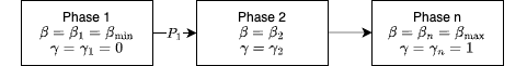
Figure 5: BLOKE parameter smoothing
Parallelization
To allow more than two BLOKE phases, we needed to parallelize our sampling processes. Luckily, only correct program rewrites are communicated between phases, which means for each adjacent phase pair, we can use a single queue as a communication medium.
As shown in Figure 6, the user will pass the initial program $x_{0}$ into the BLOKE optimizer, which would put the program into the in_queue of phase pipeline. In phase 1, we spawn off a predetermined number of sampling processes on the initial program.
Every time the sampling process of phase $n$ found a better optimization $x’$, the process will pass $x^{\prime}$ into the phase $n$ output queue to which phase $n+1$ consumes with their own sampling processes.
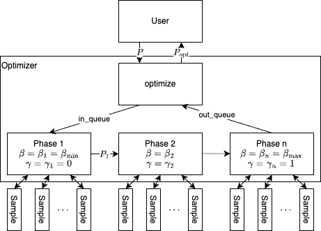 Figure 6: BLOKE parallelization
Architecture
Figure 7 shows the high-level architecture of BLOKE. The user would call the optimizer library which samples using STOKE’s random walk method. The sample library can call the Brilirs interpreter to run test cases, or call the bril_equivalence library to prove that a program in the walk is equivalent to the input program. The equivalence library would lift the Bril programs into Z3 formulas using the bril2z3 library and call Z3 to prove equivalence or find a counterexample.
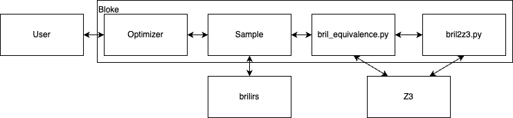 Figure 7: High level BLOKE architecture
Evaluation
We implemented BLOKE in 3200 lines of Python. We chose to not use the existing STOKE library because x86 assembly code logic was deeply entangled in its codebase.
Sadly, not many existing Bril benchmarks can be optimized with BLOKE currently since some opcodes are not supported. We support the following Bril opcodes:
const,add,mul,sub,div,eq,lt,gt,le,ge,not,and,or,jmp,br,ret,id,nop,fadd,fmul,fsub,fdiv,feq,flt,fle,fgt,fge, andphi.
BLOKE also cannot optimize programs with loops yet, which is an item for future work. So to evaluate BLOKE, we made short toy examples shown in Figure 8. clobber is shown in Figure 1.
@main(a: int,
      b: int,
      c: int): int {
  x1: int = mul a b;
  x2: int = mul a c;
  x3: int = add x1 x2;
  ret x3;
}
Figure 8a: distribute
@main(x: int): int {
  one: int = const 1;
  x: int = add x one;
  x: int = add x one;
  x: int = add x one;
  x: int = add x one;
  x: int = add x one;
  ret one;
}
Figure 8b: dead_code
@main(a: int,
      b: int): int {
  true: bool = const true;
  br true .then .else;
.then:
  ret a;
.else:
  ret b;
}
Figure 8c: unused_br
@main(x: int): int {
  one: int = const 1;
  y: int = id x;
  x: int = add x one;
  x: int = add x one;
  x: int = add x one;
  x: int = add x one;
  x: int = add x one;
  ret y;
}
Figure 8d: dead_code_alt
We measured our benchmarks on a Dell PowerEdge R620 with 62.8GiB of memory and 32 3.4GHz Intel Xeon E5-2650 v2 cores running Ubuntu 22.04.3 LTS. Each BLOKE run in our evaluation was run with 10,000 iterations.
For each benchmark, we measured the (1) performance of the optimizations BLOKE found, (2) how multiple phases affected the optimizations, (3) how fast BLOKE runs with respect to the number of processes BLOKE can have running at one time, and (4) how the number of phases impacted BLOKE runtime.
Optimization Performance
To measure the (1) performance of the optimizations BLOKE found, we ran the five benchmarks with 5 BLOKE phases and $\beta \in[1,10]$.
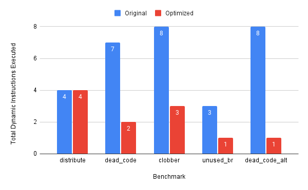 This chart shows the total number of dynamic executions executed in the original program in blue, and the number of dynamic executions executed in the optimized program in red. For most of the benchmarks we were able to find optimizations. For the ones that BLOKE found optimizations, they turned out to be the most optimal program.
We found that BLOKE did not find an optimization for the distribute benchmark (Figure 8a). The benchmark does a simple $a \cdot b+a \cdot c$, and the intent was for BLOKE to find the $a \cdot(b+c)$ identity.
@main(a: int,
      b: int,
      c: int): int {
  x1: int = add b c;
  x2: int = mul a x1;
  ret x2;
}
Figure 9: Intended distribute optimization.
We believe BLOKE was unable to find the optimization shown in Figure 9 because there are too many nonequivalent BLOKE steps to reach the intended optimization. That is, any single swap between a line in the intended optimization and a line in the original program results in an incorrect program, thereby increasing the cost of the step in the random walk. To fix this, we should run BLOKE with more sampling iterations and a lower minimum $\beta_{\text {min }}$.
Number of Phases
To measure (2) how multiple phases affected the optimization performance, we ran the five benchmarks with $\beta \in[1,10]$. We also varied the number of phases from 2 to 5.
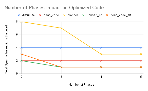 This chart shows the impact of increasing the number of phases to the improvement in the optimizations. At first glance, it looks like increasing the number of phases improved the optimizations found, and that we needed at most four phases to converge. However, this may mean we needed four times as many steps in our random walk. More investigation is definitely needed to conclude the efficacy of multiple phases on BLOKE.
Optimizer Scalability
To measure (3) how the number of phases impacted BLOKE runtime, we ran the five benchmarks with 5 BLOKE phases and $\beta \in$ $[1,10]$. We also varied the maximum number of sampling processes BLOKE can have running at a time from 1 to 32. For tractability, we gave each BLOKE trial a 30 minute timeout.
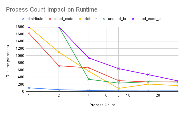 This chart show that we see a sublinear speedup for all benchmarks. The nonlinear speedup is expected because we have communication overhead from the inter-phase queues.
Number of Phases
To measure (4) how the number of phases impacted BLOKE runtime, we ran the five benchmarks with $\beta \in[1,10]$. We also varied the number of phases from 2 to 10 . For tractability, we gave each BLOKE trial a 30 minute timeout.
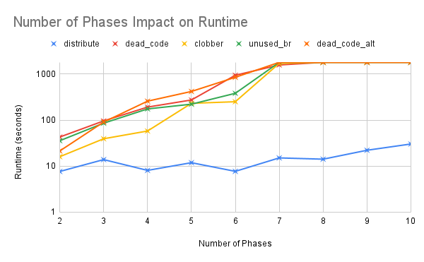 This chart shows the effects of increasing the number of phases to the optimizer runtime. As expected, as the number of phases increases, the runtime of BLOKE also increases. This is expected because the number of BLOKE sampling processes increases with respect to the number of phases we have. We hit the 30 minute timeout at around seven phases.
Another interesting observation is that for benchmarks like distribute where BLOKE is unable to find an optimization, the runtime of the optimizer is orders of seconds faster. This is likely because all BLOKE sampling processes in phase 1 produced the same program output. Had the distribute benchmark had dead code, we would likely see a similar upwards trend in runtime.
Related Works
BLOKE is based off of STOKE, a superoptimizer for loop-free x86 assembly programs. We extend STOKE to optimize programs written in an educational intermediate representation language called Bril. BLOKE use similar equivalence and performance cost functions as STOKE. In contrast to STOKE which uses a two-stage process, BLOKE allows users to specify the number of BLOKE phases $(\geqslant 2)$ for a smoother transition between the synthesis and optimization. BLOKE also uses Z3 while STOKE uses the STP theorem prover.
BLOKE is not the first project that lifts Bril to an SMT solver. Shrimp lifts Bril to SMT solvers using Rosette to prove the correctness of compiler optimization passes. Nigam et al. successfully verified the correctness of local value numbering passes using Shrimp. Rosette is an extension of the Racket programming language. BLOKE does not use Rosette since the Bril tools the autor had written previously for CS 6120 are in Python. Calling Rosette from Python is not efficient, as it currently requires subprocessing to the Racket commandline, which is expensive.
The correctness cost of BLOKE where we grow the list of testcases $\tau$ based on the counter-example output of the Z3 solver was inspired from CEGIS, or counter-example guided inductive synthesis.
Future Work
There are plenty of extensions of BLOKE. Our implementation of BLOKE has many optimization opportunities. For example, instead of Python, we can write BLOKE in a statically compiled language such as Rust or C/C++.
A natural extension BLOKE is to implement it for LLVM IR, the language Bril took its inspiration from. A common way to enforce SSA form of LLVM IR is to use memory operations, so we will need to reason about the heap in the hypothetical LLVM library.
Another immediate extension is to address the lack of compatible Bril benchmarks with support for more Bril opcodes. In particular, we should be able to model print statements and memory with the theory of arrays. It is not obvious how we would model function calls in Z3.
Since traces are loop-free, we may be able to model speculation calls and thus run BLOKE on Bril traces. We may want to implement this as an offline, feedback-directed optimizer for long-running program. Unless a subroutine in a long-running program is frequently executed, we would not want stochastic search running in a dynamic compiler in general.

Furthermore, if there is an efficient way of synthesizing some class of loop-invariants, we may be able to optimize some Bril loops.
Finally, there are exciting venues for the further distribution of BLOKE workloads using the Message Passing Interface (MPI) bindings in Python. Furthermore, during the implementation of BLOKE, we observed that a BLOKE phase is akin to a MapReduce operation, where the Map operation is the BLOKE sampling process and the Reduce is the concatenation of the outputs of each sampling process. Further work is needed to understand how different distributed algorithms such as MapReduce can be effective for BLOKE.
Conclusion
We presented BLOKE, a scalable implementation of STOKE on Bril with an extension to increase STOKE’s two-stage process of synthesis and optimization. We found that BLOKE was able to find superoptimizations of loopfree code written in Bril, an educational intermediate representation language. Furthermore, we found BLOKE to be scalable with respect to the number of cores we gave BLOKE. In short, we have found a scalable superoptimizer for an educational intermediate representation language.
Acknowledgements
We would like to thank our second monitor for providing us with much productivity.