Compilation-Based Execution Engine for a Database
My project was to implement a compilation-based execution engine for a database. The code is located here.
Introduction
Existing database systems initially convert a SQL query to a tree of relational algebra operators and then interpret that plan. In the past, this wasn't a bottleneck as the main cost of processing data was reading and writing data to disk. Since the amount of CPU time spent processing data was negligible compared to the disk access time, the overheads of interpretation didn't play a large role.
Nowadays, databases have access to faster storage and large amounts of main memory which means that the CPU time spent processing data is much more valuable. As mentioned in this overview of different execution engine implementations, "To go 10x faster, the DBMS must execute 90% fewer instructions. To go 100x faster, the DBMS must execute 99% fewer instructions." To reduce the overhead of interpretation, we can directly compile trees of operators down to binary and then execute them. This projects explores implementing such a compiler.
Background
Relational Algebra
The initial step of any database is to convert SQL to a tree of relational algebra operators.
For example, this query gets converted to the following tree of operators:
SELECT * FROM A JOIN B ON a_key = b_key WHERE x > 5
Filter(
  Join(Scan(A), Scan(b), ColRef(a_key), ColRef(b_key)),
  CompExpr(LT, ColRef(x), Literal(5))
)
The key operators needed are Scan, Select, Join and Group By/Aggregate.
Joins are implemented by creating a hash table of one of its inputs and then for each tuple of the other input, concatenating it with any matching tuple in the hash table. Similarly, grouping is done by maintaining a map of the group by values to a bucket that contains all values in the group. Then, each aggregation function is computed over each bucket.
Interpretation
Most existing databases use interpretation to generate the output. This is generally implemented by having a produce function for each operator. When you call it, the operator will call a produce function from its child operators which returns the next tuple (or null if it's done), process that tuple (filter by some condition, execute a map function, join data, etc.), and then return the processed tuple.
For example, this would be what is executed for the interpreted version of Filter(Scan(T), CompExpr(LT, ColRef(x), Literal(5))):
query {
  output = []
  while (t = op.produce()) {
    output.add(t)
  }
  return output
}

ColRef.evaluate(t) {
  return t[col]
}

CompExpr.evaluate(t) {
   l = left.evaluate(t)
   r = right.evaluate(t)
   return op(l, r);
}

Filter.produce() {
   while (t = child.produce()) {
      if (expr.evaluate(t)) {
        return t
      }
   }
}

Scan.produce() {
  return next tuple of T
}
While easy to implement from a system point of view, this leads to a lot of overhead as you have a function call boundary at each operator. This means values that are in registers need to be spilled and you have to invoke a virtual call which is expensive.
Compilation
Imagine the following equivalent code:
query {
  output = []
  for (t in T) {
    if (t[x] > 5) {
      output.add(t)
    }
  }
  return output
}
This should be much faster since there are no function calls (let alone virtual ones) and since tight loops are generated, values are kept in registers for as long as possible. Our goal is to generate code like the above and then compile and execute it.
High Level Design
Producer/Consumer Interface
To generate code for an operator tree, we introduce produce and consume functions for each operator. Produce generates a loop over the tuples in an operator's result. Consume is called by an operator's child surrounded by a loop over its result tuples. Effectively, produce signifies to "pull" tuples from an operator while consume "push"es them. Expressions have a produce function that generates code for calculating that expression. This idea comes from a paper by Thomas Neumann in 2011: "Efficiently Compiling Efficient Query Plans for Modern Hardware".
To see this in action, let's consider the following psuedocode implementations for Scan and Filter:
Scan.produce() {
  output << "for (tuple in T) {"
    parent.consume()
  output << "}"
}

Filter.produce() {
  // To generate a loop over its result, generate a loop over its child's result.
  child.produce();
}

Filter.consume() {
  // This is called in a loop over the child's result
  output << "if (";
    cond.produce()
  output << ") {"
    parent.consume()
  output << "}"
}
It's worth taking some time to appreciate how elegant this is and check that it does indeed do what we want. I was positively awestruck when I first came across it.
Special care is needed for joins and group bys since they store some of the input into a hash table and then loop over it later. Here's some psuedocode for a hash-based join:
Join.produce() {
  // First, generate a loop over one side
  left_child.produce()
  // See consume for what gets generated in that loop

  // Then, generate a loop over the other side
  right_child.produce()
  // See consume for what gets generated in that loop
}

Join.consume(src) {
  if (src == left_child) {
    // This is called in a loop over the left child's result
    output << "add t into HT"
  } else {
    // This is called in a loop over the right child's result
    output << "for (t' in HT[t]) {"
      parent.consume(this)
    output << "}"
  }
}
What is needed to make this work is for us to specialize the consume function based on which loop this is generated in. We accomplish this by invoking the consume function with the operator that generated the loop. Similarly for group by:
GroupBy.produce() {
  // First, generate a loop over child's result
  child.produce()
  // See consume for what gets generated in that loop

  // Then, loop over each bucket and then output the aggregation functions
  output << "for (bucket in HT) {"
    output << "t = compute(bucket)"
    parent.consume()
  output << "}"
}

GroupBy.consume() {
  output << "insert t into HT[group by cols of t]"
}
Implementation
I chose to focus on the compilation aspects of the project and implement just enough of the database elements to get full queries to execute.
We build up a basic storage engine by allowing user specified CSVs to be converted into our specific column files. Users can specify a catalog of these tables and column files in C++.
Queries over this catalog are written in C++ by constructing a tree of our operator classes. Then, this can be executed by invoking the code generator and then compiler on this operator tree.
Types
I map each of the SQL types to the following underlying type:
| SQL Type | Implemented Type |
|---|---|
| SMALLINT | 16-bit signed integer |
| INT | 32-bit signed integer |
| BIGINT | 64-bit signed integer |
| BOOLEAN | 8-bit boolean |
| REAL | 64-bit floating point |
| TEXT | Variable-length string |
| DATE | 64-bit signed integer containing Unix millisecond timestamp |
Storage
The file format used for a table consists of each of the columns stored as a separate file. The format of each column depends on its type:
- The format for all types except for TEXT consists of tightly-packed values of the underlying type, much like an in-memory array. No other metadata such as cardinality is stored.
- For TEXT types, the format used is as follows. The first 4 bytes represent an unsigned 32-bit integer that contains the cardinality (number of strings) inside the file. Then, for each string, we store 8 bytes. The first 4 bytes are an unsigned 32-bit integer that contains the string length. The second 4 bytes are an unsigned 32-bit integer that contains the byte offset of the string's data in the file. After this metadata array, we store all the strings in a packed format.
To avoid having to implement a buffer pool manager and on-demand paging, I mmap the column files and rely on OS paging to handle this. I simplified the experiment code behind this paper for the implementation.
Input
Since parsing and query planning/optimization are not the focus of this project, I've not implemented these. Rather, I manually enter a tree of relational algebra operators and then compile and execute that.
Operator Tree
This is fairly standard. We introduce a base Operator and Expression class that is inherited by respective implementations. Each one can hold any number of child operators or expressions.
The only thing of note is that operators need to keep track of the schema that they output. For example, a table scan would have some or all the underlying table's columns in its schema. A filter operation would have the schema of its child. A join would have the schema of the concatenation of both its inputs. A group by would have the schema of whatever aggregation functions are defined on it. To handle the general case and allow for eager removal of unnecessary columns, we associate an array of expressions as the output schema where each expression computes a function of the input schema values. While most databases implement such functionality by adding map and project operators, creating a matching expression for each column in the output schema simplifies this. I learned of this technique by looking through the implementation of NoisePage.
Code Generation
We generate C++ code directly to simplify the implementation. All the types above are native C++ types that we can reuse in the implementation. For example, we can use int16_t, int32_t and int64_t for 16, 32 and 64-bit signed integers respectively. Code is generated within a compute function, extern "C" compute() {...}.
As mentioned in the design, we use the producer/consumer interface to generate the body of this compute function. Each operator in the tree needs to have a produce/consume function on it. While initially I developed these as plain functions that simply take in an operator as input, I quickly realized that the produce and consume function calls on the same operator needed to share state. For example, the hash join produce function outputs a hash table declaration while the hash join consume function relies on that same variable.
Because state needs to be shared, we could attach these extra state variables onto the relational algebra operators. However, for better separation of concerns, we create a wrapper translator object around each operator and then organize them into the same tree. This allows for per-operator state sharing without having to modify each of the plan classes. We use the visitor pattern to generate these translator wrappers.
Each translator needs to know which variables correspond to the schema of each operator. For example, the output operator needs to know which variables correspond to each column of the child operator's schema to know which variables to push into standard out. To handle this, each translator contains a list of variables that can be queried, one for each column of its output schema.
Code Execution
Once the C++ file has been generated, we invoke clang on the file with optimizations turned on (-O3). We allow any C++ header defined in the codebase to be included. This enables us to reuse classes defined in the codebase such as the ones for file reading. This generates a dynamic library that we load into the database with dlopen. We retrieve the aforementioned compute function via dlsym and then execute it. Finally, we dlclose the dynamic library.
Performance Evaluation
Benchmark Suite
The specific benchmark suite I'm using is the TPC-H benchmark. The schema can be found in my code base in tpch/schema.sql. The underlying data is generated by an automated tool. This tool has various scale factors to run the queries at. Scale factor 1 means there is a total of 1 GB of data, 10 means 10 GB of data and so on. I'm running these experiments on my rather underpowered (and out of disk space) laptop so I ran it at scale factor 1.
The queries involved are a mix of filters, group/by aggregations and joins. I've selected a set of 5 queries out of the whole benchmark to run the compiler on (queries 1, 3, 6, 11 and 12). These queries are unchanged except for the removal of subqueries, order by and having clauses as I don't support them. The remaining queries were mostly the same with those removed so I chose to omit them since I had to manually convert them to a physical query plan.
Baseline
Postgres is a popular database that uses an interpretation-style execution engine so I thought it was fit to compare against as a baseline. Since my code is single-threaded, I set max_parallel_workers to 1. I also set jit off. Postgres includes a very basic compiler that will generate LLVM code for expressions only and not operators. However, since I am interested in comparing against the interpretation version, I set this off. I'm running Postgres 13.
Postgres does store full table tuples packed on disk while I store them separately. This does mean we load less data which gives us an unfair advantage. To fix this, I created materialized views of each of the base tables with only the relevant loaded columns. For example, for Q1:
CREATE TABLE lineitem_01 AS (SELECT l_returnflag, l_linestatus, l_quantity, l_extendedprice, l_discount, l_tax, l_shipdate FROM lineitem);
Then, you can rewrite the query to use this newly created lineitem_01 table. This way, Postgres and our system read the same amount of data from disk.
I also verify correctness by checking that the query results are identical in Postgres.
Setup
I'm running this on a MacBook Pro, Late 2013 with an i7-4750 HQ and 8GB of RAM. This is running Ubuntu 20.04 under the Windows Linux Subystem 2.
For both systems, I took total running times on the client. This means it includes time to print the result rows but I redirected stdout to /dev/null. While this does include time to execute query planning for Postgres, Postgres reports that it takes less than a millisecond for these on all queries so I've omitted values beyond the decimal place to account for the loss of accuracy.
Results
None of the queries had a correctness error.
I ran 4 trials for each query and report the 95% (t-statistic) confidence intervals for the runtime. I report two columns for my system, one with the compile times omitted (so just the time spent actually processing the query) and also the total time for compilation and execution.
| Query | Postgres Interval (ms) | KushDB Execution Only Interval (ms) | KushDB Total Interval (ms) |
|---|---|---|---|
| Q1 | 2027 - 2332 | 192 - 466 | 1061 - 1611 |
| Q3 | 818 - 1253 | 562 - 617 | 1771 - 2052 |
| Q6 | 434 - 684 | 63 - 68 | 762 - 1502 |
| Q11 | 118 - 186 | 28 - 118 | 1186 - 1554 |
| Q12 | 506 - 696 | 105 - 114 | 922 - 1262 |
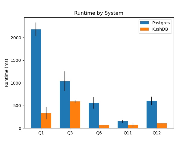
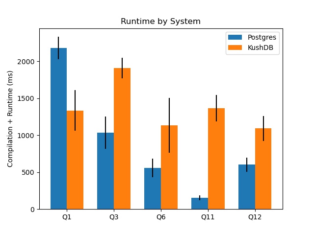
For all queries, the compilation version (once compiled) greatly outperforms Postgres or matches it in the case of Q11. I suspect that the noise of measurement outweights any improvement in runtime given how fast both systems execute the query. However, once we take into account the compilation time, a different result emerges.
Compilation Time
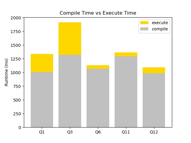
At such low table sizes, the time spent compiling actually dominates. Note that the time spent compiling is fixed so as the database size grows larger, the yellow portion of the graph will increase and the grey portion will stay constant. This means the ratio of time spent compiling to time spent executing will decrease on larger databases.
However, this is still unacceptable on smaller data sets where Postgres outperforms the compilation version. In future work, I discuss some ways that this can be fixed.
Personal Experiences
The largest barrier I had to overcome in working on this project was understanding all the pieces of the puzzle:
- While I theoretically knew how to implement paging and learned about it in detail in both databases and operating systems courses, I needed to do enough research to figure out which syscalls to use.
- I also knew of dynamic libraries but it took some time to figure out exactly how to load in a shared library and access functions within it.
I also gained valuable experience building up a codebase that can easily scale. As an example, once I built in the functionality and infrastructure to specify arbitrary types, I could add in new types to the system with only 3 lines of additional code.
Future Work
While this generates extremely high performant code, the time spent compiling is extremely large. The following strategies are useful in reducing this:
- Directly generate some IR. This removes any overhead for file I/O to output the C++ and parsing, type checking and lowering that C++ to IR. The paper mentioned above, by Thomas Neumann, directly generates LLVM. However, a recent paper from his research group, "Tidy Tuples and Flying Start: Fast Compilation and Fast Execution of Relational Queries in Umbra" by Timo Kersten, Viktor Leis and Thomas Neumann, describes how they move to a custom IR. While they noted that "LLVM IR is designed to be more generic to support a wide variety of optimization passes", they also "found that [LLVM's] flexibility is counter-productive for query latency" as it "has an emphasis on instruction reordering, replacement, and deletion". This matches the conventional wisdom that led to development of simpler code generators like DynASM, B3, and Cranelift. Similar to JITs, Umbra also adaptively switches from interpreting IR to converting IR to binary and executing that.
- Control which optimization passes run on this. For example, most of the overhead comes from dead copies that get inserted into the code. One GVN/DCE pass can get rid of these. Auto-vectorization would also prove beneficial here.
As always, there are a myriad of SQL features that I have not implemented as part of this project. Adding more features would allow me to test this more thoroughly.
Another aspect to explore is how best to parallelize the generated code. Existing techniques break the code up into the materialization boundaries and then use simple strategies to parallelize it.
Finally, to simplify the codebase, we can take advantage of operator overloading to define proxy types. For example, if you have ints a and b, writing a * b in your source code generates code that multiplies a and b. One more layer of indirection will simplify this. For example, if you have proxy[int]s a and b, writing a * b in your source code generates code that generates a program that multiplies a and b. This technique was popularized by the LMS project and is used by a few database systems like LegoBase and LB2. This technique allows you to write code that behaves like the compilation version but appears like the interpreted version, making development easier.