The instructor is extremely thankful to Prof. Steve Seitz for allowing us to use this project which was developed in his Computer Vision class.

Synopsis

In this project, you will write code to detect discriminating features in an image and find the best matching features in other images.  Your features should be reasonably invariant to translation, rotation, illumination, and scale, and you'll evaluate their performance on a suite of benchmark images.  We'll rank the performance of features that students in the class come up with, and compare them with the current state-of-the-art.

In Project 2, you will apply your features to automatically stitch images into a panorama. 

To help you visualize the results and debug your program, we provide a working user interface that displays detected features and best matches in other images.  We also provide sample feature files that were generated using SIFT, the current best of breed technique in the vision community, for comparison.

Description

The project has three parts:  feature detection, description, and matching.

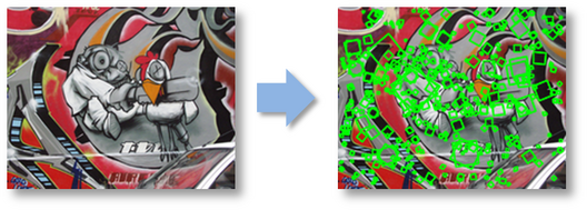
1. Feature detection

In this step, you will identify points of interest in the image using the Harris corner detection method.  The steps are as follows (see the lecture slides/readings for more details)  For each point in the image, consider a window of pixels around that point.  Compute the Harris matrix H for that point, defined as

where the summation is over all pixels p in the window.  The weights should be chosen to be circularly symmetric (for rotation invariance).  A common choice is to use a 3x3 or 5x5 Gaussian mask. Note that these weights were not discussed in the lecture slides, but you should use them for your computation.

Note that H is a 2x2 matrix.  To find interest points, first compute the corner strength function

Once you've computed c for every point in the image, choose points where c is above a threshold.  You also want c to be a local maximum in at least a 3x3 neighborhood (we found that 5x5 window works better). In addition to computing the feature locations, you'll need to compute a canonical orientation for each feature, and then store this orientation (in radians) in each feature element.

2. Feature description

Now that you've identified points of interest, the next step is to come up with a descriptor for the feature centered at each interest point.  This descriptor will be the representation you'll use to compare features in different images to see if they match.

You will implement 3 descriptors for this project. For starters, you will implement a simple descriptor, a 5x5 square window without orientation. This should be very easy to implement and should work well when the images you're comparing are related by a translation. Next, you'll implement a simplified version of the MOPS descriptor. You'll compute an 8x8 oriented patch sub-sampled from a 41x41 pixel region around the feature.

Finally, you will implement your own feature descriptor.  You can define it however you want, but you should design it to be robust to changes in position, orientation, and illumination.  You are welcome to use techniques described in lecture (e.g. using image pyramids), or come up with your own ideas.

3. Feature matching

Now that you've detected and described your features, the next step is to write code to match them, i.e., given a feature in one image, find the best matching feature in one or more other images.  This part of the feature detection and matching component is mainly designed to help you test out your feature descriptor.  You will implement a more sophisticated feature matching mechanism in the second component when you do the actual image alignment for the panorama.

The simplest approach is the following:  write a procedure that compares two features and outputs a distance between them.  For example, you could simply sum the absolute value of differences between the descriptor elements. You could then use this distance to compute the best match between a feature in one image and the set of features in another image by finding the one with the smallest distance. Two possible distances are:

1.  use a threshold on the match score. This is called the SSD distance, and is implemented for you as match type 1, in the function ssdMatchFeatures.
2.  compute (score of the best feature match)/(score of the second best feature match). This is called the "ratio test"; you must implement this distance.

Testing

Now you're ready to go!  Using the UI and skeleton code that we provide, you can load in a set of images, view the detected features, and visualize the feature matches that your algorithm computes.

We are providing a set of benchmark images to be used to test the performance of your algorithm as a function of different types of controlled variation (i.e., rotation, scale, illumination, perspective, blurring).  For each of these images, we know the correct transformation and can therefore measure the accuracy of each of your feature matches.  This is done using a routine that we supply in the skeleton code.

You should also go out and take some photos of your own to see how well your approach works on more interesting data sets.  For example, you could take images of a few different objects (e.g., books, offices, buildings, etc.) and see if it can "recognize" new images.

Skeleton Code

Follow these steps to get started quickly:

1.   Download the skeleton code here.
This skeleton code should compile under Windows (Visual Studio) or Linux (with the provided Makefile). Note that under Linux you may need to install a few packages, including FLTK (for the UI), libjpeg, and libpng. Under Ubuntu, these packages are currently called 'libfltk1.1-dev', 'libjpeg62-dev', and 'libpng12-dev'.

Note that you are free to implement this project entirely in Matlab (as long as you write the Harris detector and matching routines yourself).

The project has also been compiled under Mac (thanks to Daniel Cabrini Hauagge for the following instructions):

1. Install MacPorts (free and opensource package manager).
2. Install fltk using MacPorts (just run "sudo port install fltk" on the command line)
3. Install libpng using MacPorts ("sudo port install libpng")
4. Install libjpeg from http://www.ijg.org/ (to compile do: ./configure; make; make test; sudo make install)
5. Replace "Makefile" with this one for mac.

2.      Download some image sets for plotting ROC curves: graf, Yosemite.
Included with these images are some SIFT feature files and image database files.

3.      Download some image sets for benchmark: graf, leuven, bikes, wall
Included with these images are some SIFT feature files and image database files.

4.      Download the solution EXE here (Win32) or here (Linux) or here (Mac). (You might need to use "chmod" first to make it executable on Linux or Mac.)

After compiling and linking the skeleton code, you will have an executable Features This can be run in several ways:

• Features

with no command line options starts the GUI. Inside the GUI, you can load a query image and its corresponding feature file, as well as an image database file, and search the database for the image which best matches the query features. You can use the mouse buttons to select a subset of the features to use in the query.

Until you write your feature matching routine, the features are matched by minimizing the SSD distance between feature vectors. This can be changed by selecting the appropriate matching algorithm menu item. Note that since no threshold is defined in the UI, the results of both matching algorithms will be identical.

• Features computeFeatures imagefile featurefile [featuretype descriptortype]
  uses your feature detection routine to compute the features for imagefile, and writes them to featurefile. featuretype specifies which type of feature detector to use(1 is for a very simple detector, 2 is for your Harris detector, and 3 onwards is for optrional detectors you choose to implement); descriptortype specifies which type of descriptor to compute (1 is for the simple feature descriptor, 2 is for your MOPS descriptor, and 3 is for your custom descriptor).
• Features matchFeatures featurefile1 featurefile2 threshold matchfile [matchtype]
  takes in two sets of features, featurefile1 and featurefile2 and matches them using your matching routine (the matching routine to use is selected by [matchtype]; 1 (SSD) is the default, and 2 uses your ratio distance). The threshold for determining which matches to keep is given by threshold. The results are written to a file, matchfile, which can later be read by the Panorama program.
• Features matchSIFTFeatures featurefile1 featurefile2 threshold matchfile [matchtype]
  same as above, but uses SIFT features.
• Features roc  featurefile1 featurefile2 homographyfile [matchtype] rocfile aucfile
  creates the points necessary for the ROC curve for the feature you implement. You will use these values to create plots for your ROC curves. It also computes the area under the ROC curve (AUC) and writes it a file.
• Features rocSIFT  featurefile1 featurefile2 homographyfile [matchtype] rocfile aucfile
  is the same as above, but uses the SIFT file format.
• Features benchmark imagedir [featuretype descriptortype matchtype]
  tests your feature finding and matching for all of the images in one of the four above sets. imagedir is the directory containing the image (and homography) files. This command will return the average pixel error and average AUC when matching the first image in the set with each of the other five images.  

To Do

We have given you a number of classes and methods to help get you started. The only code you need to write is for your feature detection methods, your descriptor computing methods and your feature matching methods, all in features.cpp. Then, you should modify computeFeatures and matchFeatures in the file features.cpp to call the methods you have written.  We have provided a function dummyComputeFeatures that shows how to create the code to detect features, as well as integrate it into the system. You'll need to complete ComputeSimpleDescriptors and implement ComputeMOPSDescriptors and ComputeCustomDescriptors. These 3 functions take the information already stored in features and compute descriptors for feature points, then they store such descritpors in the data field of features. The function ssdMatchFeatures implements a feature matcher which uses the SSD distance, and demonstrates how a matching function should be implemented.  The function ComputeHarrisFeatures is the main function you will complete, along with the helper functions computeHarrisValues and computeLocalMaxima.  You will also implement the function ratioMatchFeatures for matching features using the ratio test.

After you've finished computeFeatures part of this project. You may use UI to perform individual queries to see if things are working right. First you need to load a query image, and then its corresponding feature file with .f extension. Then, you'll need to load another file's database file, which is simply a .db file containing one line 'imagename featurefilename \n'. Note that the newline symbol is crucial. Then, select a subset of features individually (left-click) or in a group (right-click drag) and perform query, you should be able to see another image with matched features showing up to the right of query image.

You will also need to generate plots of the ROC curves and report the areas under the ROC curves (AUC) for your feature detecting and matching code (using the 'roc' option of Features.exe), and for SIFT. For both the Yosemite test images (Yosemite1.jpg and Yosemite2.jpg), and the graf test images (img1.ppm and img2.ppm), create a plot with 8 curves, three using the simple window descriptor , simplified MOPS descriptor and your own feature descriptor with the SSD distance, three using such 3 types of descriptors with the ratio test distance, and the other two using SIFT (with both the SSD and ratio test distances; these curves are provided to you in the zip files for Yosemite and graf provided above).

We have provided scripts for creating these plots using the 'gnuplot' tool. Gnuplot is installed on the lab machines, at 'C:\Program Files\gnuplot\binaries\wgnuplot.exe' ('gnuplot' is also available as an Ubuntu or MacPorts package)  or you can download a copy of Gnuplot to your own machine. To generate a plot with gnuplot (using a gnuplot script 'script.txt', simply run 'C:\Program Files\gnuplot\binaries\wgnuplot.exe script.txt', and gnuplot will output an image containing the plot. The two scripts we provide are:

plot.roc.txt: plots the ROC curves for the SSD distance and the ratio test distance. These assume the two roc datafiles are called 'roc1.txt' (for the SSD distance), and 'roc2.txt' (for the ratio test distance). You will need to edit this script if your files are named differently. This script also assumes 'roc1.sift.txt' and 'roc2.sift.txt' are in the current directory (these files are provided in the zip files above). This script generates an image named 'plot.roc.png'. Again, to generate a plot with this script, simply enter 'C:\Program Files\gnuplot\binaries\wgnuplot.exe plot.roc.txt'.

plot.threshold.txt: plots the threshold on the x-axis and 'TP rate - FP rate' on the x-axis. The maximum of this function represents a point where the true positive rate is large relative to the false positive rate, and could be a good threshold to pick for the computeMatches step. This script generates an image named 'plot.threshold.png.'

Finally, you will need to report the average AUC for your feature detecting and matching code (using the 'benchmark' option of Features.exe) on four benchmark sets : graf, leuven, bikes and wall.

 

What to Turn In

First, your source code and executable should be zipped up into an archive called 'code.zip', and uploaded to CMS. In addition, turn in a web page describing your approach and results.  In particular:

• Describe your feature descriptor in enough detail that some one could implement it from your write-up
• Explain why you made the major design choices that you did
• Report the performance (i.e., the ROC curve and AUC) on the provided benchmark image sets

1.        You will need to compute two sets of 8 ROC curves and post them on your web page as described in the above TO DO section. You can learn more about ROC curves from the class slides and on the web here and here.

2.        For one image each in both the Yosemite and graf test pairs, please include an image of the Harris operator on your webpage.  This image is produced by the Features.exe executable every time it is run in computeFeatures mode (it is saved to the file harris.tga). If these images seem too dark, you can multiply the Harris score by a constant, such as 2, to make the scores more visible.

3.        Report the average AUC for your feature detecting (simple 5x5 window descriptor, MOPS descriptor and your own new descriptor) and matching code (both SSD and ratio tests) on four benchmark sets graf, leuven, bikes and wall. 

• Describe strengths and weaknesses
• Take some images yourself and show the performance (include some pictures on your web page!)
• Describe any extra credit items that you did (if applicable)

 

We'll tabulate the best performing features and present them to the class.

The web-page (.html file) and all associated files (e.g., images, in JPG format) should be placed in a zip archive called 'webpage.zip' and uploaded to CMS. If you are unfamiliar with HTML you can use any web-page editor such as FrontPage, Word, or Visual Studio 7.0 to make your web-page. Here are some tips.

Extra Credit

Here is a list of suggestions for extending the program for extra credit. You are encouraged to come up with your own extensions as well!

• Implement adaptive non-maximum suppression (MOPS paper)
• Make your feature detector scale invariant.
• Implement a method that outperforms the above ratio test for deciding if a feature is a valid match.
• Use a fast search algorithm to speed up the matching process.  You can use code from the web or write your own (with extra credit proportional to effort).  Some possibilities in rough order of difficulty:  k-d trees (code available here), wavelet indexing (approach from lecture),  locality-sensitive hashing.

 

Last modified on Feburary 7, 2011