Nori an educational ray tracer
About
Nori is a simple ray tracer written in C++. It runs on Windows, Linux, and Mac OS and provides basic functionality that is required to complete the projects in CS6630.
While Nori provides much support code to simplify your development work as much as possible, the code that you will initially receive from us in fact does very little: it renders a simple scene with ambient occlusion and writes the output image to an OpenEXR file. Your task will be to extend this system to a full-fledged physically-based renderer as part of programming assignments and your final project.
Nori was designed by Wenzel Jakob and Steve Marschner.
Core features
The Nori base code provides/will provide the following:- XML-based scene loader
- Basic point/vector/normal/ray/bounding box classes
- Pseudorandom number generator (Mersenne Twister)
- Deterministic n-dimensional integrator (cubature)
- χ2- and t-tests to verify sampling code
- Simple GUI to watch images as they render
- Support for saving output as OpenEXR files
- Loader for Wavefront OBJ files
- SAH kd-tree builder and traversal code
- Ray-triangle intersection
- Image reconstruction filters
- Code for multithreaded rendering
Documentation
Getting Nori
The source code of Nori is available on github. For details on git in general, please refer to github's Introduction to Git. To check out a copy of the source code, enter
$ git clone git://github.com/wjakob/nori.git
on the terminal (or use TortoiseGit on Windows). Note that we'll publish extensions and bugfixes to this repository, so remember to pull changes from it every now and then.
Compiling it
Nori depends on Qt, Boost, and OpenEXR. Please first install these libraries on your system and make sure that they can be found by the compiler (they must be on its header and library search path). Because building OpenEXR on Windows can be quite tricky, we provide precompiled binaries for Visual Studio 2010. Another dependency is the Eigen linear algebra library, which you do not need to install.
With the dependencies in place, run one of the following commands inside the Nori directory:
$ qmake                                           # (on Linux)
$ qmake -spec macx-g++                            # (on Mac OS X)
$ qmake -tp vc                                    # (on Windows)
On Linux and Mac OS, this will create a Makefile, and on Windows it will create a Microsoft Visual C++ project. The rest should be as simple as running make or compiling the project in Visual Studio (remember to switch to a x64/Release build). Afterwards, you can launch the renderer with a test scene, e.g.
$ ./nori scenes/cbox/cbox.xml
Note that the above syntax may vary slightly depending on your operating system.
Getting started with the code
Eigen
When developing any kind of graphics-related software, it's crucially important to be familiar with the core mathematics support library that is responsible for basic linear algebra types, such as vectors, points, normals, and linear transformations. Nori uses Eigen 3 for this purpose, which is an amazing and somewhat mysterious set of C++ header files that provides all of these primitives (and much more) based on a technique called expression templates.
We don't expect you to understand the inner workings of this library but recommend that you at least take a look at the tutorial provided on the Eigen web page. One consequence of using expression templates is that you will often write code that looks surprisingly inefficient. For instance, to check whether the components of the transposed matrix-vector product ATb are less than zero, one could write:
if (((A.transpose() * b).array() < 0).all()) { ... }
Which looks as though it will create many unnecessary copies of objects. However, the expression template machinery will ensure that this in fact compiles to highly optimized machine code.
Nori provides a set of linear algebra types that are derived from Eigen's matrix/vector class (see the header file include/nori/vector.h). This is necessary because we will be handling various quantities that require different treatment when undergoing homogeneous coordinate transformations, and in particular we must distinguish between positions, vectors, and normals. The main subset of types that you will most likely use are:
- Point2i,
- Point2f,
- Point3f,
- Vector2i,
- Vector2f,
- Vector3f, and
- Normal3f.
Nori code
When working with Nori code, it is advisable to configure your editor so that it uses tabs of length 4 to format the source code. Otherwise, the indentation will be incorrect, making the code difficult to read.
Take a moment to browse through the header files in include/nori. You will generally find all important interfaces and their documentation in this place. The most important class there is called NoriObject — it is essentially the base class of everything that can be constructed using the XML scene description language. Other interfaces (e.g. Camera) derive from this class and expose additional more specific functionality (e.g. to generate an outgoing ray in the case of a camera).
You will notice that much of the code uses templates to be oblivious to the number of dimensions and data types. Sometimes it is useful to test new algorithms in one or two dimensions, or with higher precision, and these generic classes allow doing just that.
API documentation generated by Doxygen is available here
Construction alert!
Nori is a brand-new piece of software developed just for this course. It's quite possible that you'll encounter bugs or other rough edges. We appreciate any kind of feedback so that it can be improved.
Scene file format and parsing
Nori uses a very simple XML-based scene description language, which can be interpreted as a sort of building plan: the parser creates the scene step by step as it reads the scene file from top to bottom. The XML tags in this document are essentially requests to construct certain C++ objects, with additional information on how to put them together.
Each XML tag is either an object or a property. Objects correspond to C++ instances that will be allocated on the heap. Properties are small bits of information that are passed to an object at the time of its instantiation. For instance, the following snippet creates red diffuse BSDF:
- <bsdf type="diffuse">
- <color name="albedo" value="0.5, 0, 0"/>
- </bsdf>
Here, the <bsdf> tag will cause the creation of an object of type BSDF, and the type attribute specifies what specific subclass of BSDF should be used. The <color> tag creates a property of name albedo that will be passed to its constructor.
If you open up the file src/diffuse.cpp, you will see that there is a constructor, which looks for this specific property:
- Diffuse(const PropertyList &propList) {
- m_albedo = propList.getColor("albedo", Color3f(0.5f));
- }
The piece of code that associates the "diffuse" XML identifier with the Diffuse class in the C++ code is a macro found at the bottom of the file:
- NORI_REGISTER_CLASS(Diffuse, "diffuse");
Certain objects can be nested to construct hierarchies. For example, the following snippet creates a mesh that loads its contents from an external OBJ file and assigns a red diffuse BRDF to it.
- <mesh type="obj">
- <string type="filename" value="bunny.obj"/>
- <bsdf type="diffuse">
- <color name="albedo" value="0.5, 0, 0"/>
- </bsdf>
- </mesh>
Implementation-wise, the nesting will cause a method named addChild() to be invoked within the parent object. In this specific example, this means that Mesh::addChild() is called, which roughly looks as follows:
- void Mesh::addChild(NoriObject *obj) {
- switch (obj->getClassType()) {
- case EBSDF:
- if (m_bsdf)
- throw NoriException(
- "Mesh: multiple BSDFs are not allowed!");
- /// Store pointer to BSDF in local instance
- m_bsdf = static_cast<BSDF *>(obj);
- break;
- // ..(omitted)..
- }
The following different types of properties can currently be passed to objects within the XML description language:
- <boolean name="property name" value="true/false"/>
- <float name="property name" value="float value"/>
- <integer name="property name" value="integer value"/>
- <string name="property name" value="arbitrary string"/>
- <point name="property name" value="x, y, z"/>
- <color name="property name" value="r, g, b"/>
Linear transformations are also supported, but their syntax is slightly different:
- <transform name="property name">
- <!-- Any sequence of the following operations: -->
- <translate value="x, y, z"/>
- <scale value="x, y, z"/>
- <rotate axis="x, y, z" angle="deg."/>
- <!-- Useful for cameras and spot lights: -->
- <lookat origin="x,y,z" target="x,y,z" up="x,y,z"/>
- </transform>
The top-level element of any scene file is usually a <scene> tag, but this is not always the case. For instance, in the first assignment you will run statistical tests on BRDF models, and these tests are also specified using the XML scene description language.
- <?xml version="1.0"?>
- <test type="chi2test">
- <!-- Run a χ2 test on the microfacet BRDF
- model (@ 0.01 significance level) -->
- <float name="significanceLevel" value="0.01"/>
- <bsdf type="microfacet">
- <float name="alpha" value="0.1"/>
- </bsdf>
- </test>
Guidelines
Working in groups
We recommend that you work in groups of two or three students. Larger groups are unlikely to work effectively, and doing everything alone will be quite stressful.
Before you start to work on an assignment, it is important to figure out how to partition it into reasonably-sized pieces that can be developed by different group members, in parallel. This will require some initial planning to sketch out interfaces and data structures that the different components will require to interact with each other. Shirking the planning stage brings with it the risk of doing a lot of unproductive work, so we recommend that you take it seriously.
For smaller projects, pair programming may be a more effective development model. This usually involves creating a specification off-line and then taking turns at writing code and checking that the code meets the specification.
If you require help in finding a partner, please notify the course staff, and we'll be happy to pair you up with someone in the course.
Permissible sources of information
Feel free to consult additional references when completing projects, but remember cite them in your writeup.
When asked to implement feature X, we request that you don't go and read the source code of the implementation of X in some other renderer, because you will learn little in the process. The PBRT book is excluded from this rule. If in doubt, get in touch with the course staff.
References
You may find the following general references useful:
- "Physically Based Rendering, Second Edition: From Theory To Implementation" by Matt Pharr and Greg Humphreys. Morgan Kaufmann, 2nd edition, July 2010.
- "Advanced Global Illumination" by Philip Dutré, Philippe Bekaert, and Kavita Bala. AK Peters, 2nd edition, August 2006.
- "Robust Monte Carlo Methods for Light Transport Simulation ", PhD Thesis by Eric Veach, Stanford University, December 1997.
What to submit?
We will generally inspect but not manually test your submitted code, so it's your job to convince us that it does what it's supposed to do. In addition to the specific requirements of each project, you should therefore also turn in a writeup (as a PDF file) with the following information:
Metadata
- The project title — e.g. "Homework 2: Monte Carlo sampling and statistical hypothesis tests"
- The names and NetIDs of all students in the group submitting the project
- Who did what, i.e. how you distributed work amongst group members.
Summary
Summarize the most noteworthy aspects of the rest of your overview. Anything you mention here should be described in more detail later in the document. You might include:- Which parts of the project were the most challenging.
- Interesting design decisions that you made.
- Major issues that you ran into while designing, implementing, or testing your submission.
- Known problems with your implementation, such as missing functionality or bugs.
Design and Implementation
Discuss how you created a program that satisfies the project specification. This includes topics such as:- What classes you created and why.
- What algorithms and/or data structures you used. We encourage you to include high-level pseudocode of any complex algorithms. We also encourage discussion of any boundary conditions or formulas involved, as well as citations for sources of your algorithms.
- Tradeoffs you made between simplicity of code and efficiency of execution.
- How you verified the correctness of your implementation.
You may find it useful to develop this section of the writeup in parallel with your code. When you work out an algorithm or formula that goes into your code, document it and explain it here, for yourself, before you forget how you derived it—then your writeup will be half done already.
Comments
We would appreciate any comments or criticism to improve the projects in future years. This section of the overview document will not be graded. For instance:- How much time did you spend on the assignment? How was it divided between designing, coding, and testing?
- What advice should we have given you before you started?
- What was hard or surprising about the assignment?
- What did you like or dislike? What else would you change?
Introduction
Microfacet theory is a framework for describing scattering from rough surfaces by modeling them as an arrangement of a large number of small flat "microfacets" with mirror-like reflection. This is often a good approximation for a surface that is rough at a scale small relative to the size of the pixels in an image but still large relative to the wavelengths of light.
In this assignment, you will implement a classic microfacet BRDF model and use statistical hypothesis tests to make sure that you have, in fact, created a correctly working implementation. To keep the project manageable, we won't render any images with this model yet, but you'll be able to make full use of your implementation in the next project.
The framework code provided to you comes with an implementation of a diffuse BRDF, and test harnesses that can perform χ2- and t-tests on any BSDF model that implements the required C++ interface. Your first task will be to compile the code and check that the diffuse material implementation passes both of these tests on your machine. You can do this by running the commands
$ ./nori scenes/tests-hw2/chi2test-diffuse.xml
$ ./nori scenes/tests-hw2/ttest-diffuse.xml
in the main Nori directory. Note that at this point in time, the framework is still quite concise. Many components are still missing, in particular all of the ray intersection and rendering code. Before diving into the assignment, we therefore suggest that you make use of this opportunity to browse through the code and make sure that you roughly understand how it works.
1. Microfacet BRDF
Take a look at the files include/nori/bsdf.h, src/diffuse.cpp, and src/microfacet.cpp. The latter contains some code for loading parameters and setting up the internal state of the microfacet reflectance model, but all evaluation and sampling code currently throws exceptions.
Your task is to develop the missing pieces. The microfacet BRDF you'll implement is a sum of a diffuse lobe and a glossy microfacet reflectance lobe:
fs(ωi,ωo)=kdπ+ksD(hr)F(ωi⋅hr)G(ωi,ωo,hr)4|ωi⋅n||ωo⋅n|
where hr=(ωi+ωo)/‖ denotes the half-direction vector, D is the Beckmann microfacet distribution, F is the Fresnel reflectance and G is a rational approximation of the shadowing-masking term discussed in class. The factors k_s and k_d specify the relative weight of the specular and diffuse components, and for energy conservation we require that k_s+k_d\le 1.
A thorough review of this model, including methods for importance sampling it, is contained in the paper Microfacet Models for Refraction through Rough Surface by Walter et al. The main change between our version and the model in the paper is that we have a diffuse component and ignore refraction. Furthermore, we will only use the Beckmann distribution (so you can skip the paper sections on refraction, and the Phong and GGX distributions). Beware of missing or superfluous cosine factors.
This BRDF is great for modeling materials such as plastic or lacquer, as well as other things that are diffuse-ish but also have a strong specular component. However, in terms of the underlying physics, the way that the diffuse component of f_s currently works is not particularly realistic. If you would like a little extra challenge, get in touch with us, and we'll provide you with suggestions on how the model can be further improved.
2. Monte Carlo sampling
In a Monte Carlo renderer, it is important to have random distributions available that approximate the BRDFs in the scene. This means an implementation of a BRDF has several jobs: not only do you need to be able to evaluate the BRDF f_s(\omega_i, \omega_o), but you also need to be able to randomly generate directions \omega that are distributed according to a pdf p(\omega) that resembles f_s(\omega_0, \omega) for some fixed \omega_0. In order to use these random samples, you also have to know the probability density with which these directions are generated.
In Nori, BSDF::eval() evaluates the f_s, BSDF::sample() generates random directions, and BSDF::pdf() computes the probability density (with respect to the solid angle measure) with which a given direction is generated by sample(). The sample() function also returns a sampling weight, which is the ratio of BRDF-times-cosine to the probability density. Implementing the microfacet BRDF in Nori boils down to implementing these three functions for the Microfacet subclass.
3. Testing
Once you feel like you might have a working implementation, it's time to put it to the test! For that purpose, we're providing you with two types of statistical tests that attempt to validate different parts of your implementation.
χ2-test
The first is the χ2 test discussed in class, which verifies that the sample() method provided by your implementation really has the distribution that it claims to have (i.e. the one provided by pdf()). To run this test for a few different material configurations, execute the following command:
$ ./nori scenes/tests-hw2/chi2test-microfacet.xml
Below is an example snippet of the output that appears when running the χ2 test on a correct implementation of the microfacet model.
Testing: Microfacet[
  alpha = 0.6,
  intIOR = 1.8,
  extIOR = 1.3,
  kd = [0.4, 0.2, 0.3],
  ks = 0.769231
]
Accumulating 1000000 samples into a 10x20 contingency table ..
Integrating expected frequencies ..
Writing current state to chi2test_19.m
Chi-square statistic = 91.9314 (d.o.f. = 99)
Accepted the null hypothesis (p-value = 0.679798, significance level = 0.000502408)
When the χ2-test finds a discrepancy in your sampling code (i.e. when it rejects the null hypothesis that your sampling code produces the right distribution), the best way to start debugging the issue is by inspecting the internal tables used by the test. For this reason, it writes out a MATLAB-compatible file for every conducted test with the filename chi2test_<number>.m.
Upon running one of these files in MATLAB you'll get a plot like similar to the following:
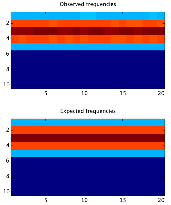
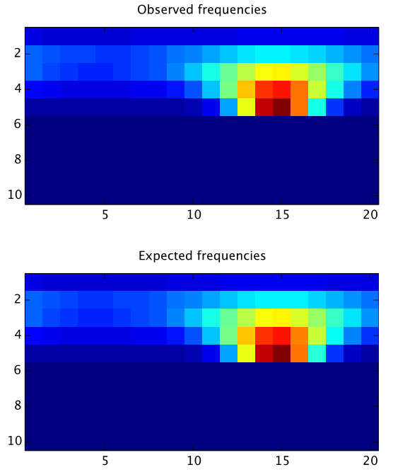
The upper plot is a histogram obtained by calling sample() many times, and "binning" the directions in spherical coordinate space. The bottom plot specifies the expected number of samples per bin, which is computed by numerically integrating your pdf() function over rectangles in spherical coordinate space. This is internally done using a Genz-Malik cubature rule.
Obviously, the two should match as closely as possible, but how can one judge when a match is "good enough"? This is where statistical tests become extremely useful, because they allow quantifying the uncertainties in such comparisons. In practice, these tests are often remarkably reliable in detecting bugs, even when a visual comparison of the two different histograms does not reveal any noticeable differences.
Student's t-test
The previous test only cared about the directional distribution of samples and completely ignored the importance weight returned by sample(). For this reason, we're providing you with a second test to ensure that certain integrals over your BRDF model converge to the right value, and this test will cover the remaining code.
Observe that under uniform incident illumination of L_i=1\frac{W}{m^2\,sr}, the reflected radiance in direction \omega_o is given by
L_r(\omega_o)=\int_{H^2}f_s(\omega_i,\omega_o)\,\cos\theta_i\,\mathrm{d}\sigma(\omega_i)
Our test approximates this function for a few different angles of incidence using Monte Carlo integration, i.e. it computes sums
\widehat {L_r}(\omega_o)=\sum_{k=1}^N\, \frac{f_s(\vartheta_k,\omega_o)}{p(\vartheta_k)}\,\cos(\vartheta_k, N)
where \vartheta_i is distributed according to the importance sampling density function p. As it happens, the summed expression is exactly what's implemented by your sample() function, so the computation just involves calling this function many times and averaging the returned values. The resulting mean is then compared against a reference value provided by us.
Because this comparison is inherently contaminated with noise, we again arrive at the question of whether or not a deviation from the reference can be taken as evidence for an implementation error, except that we're now dealing with just a single random variable instead of an entire distribution.
Our strategy will be to obtain estimates of the mean and variance of this random variable \widehat{L_r}, which are then used to run Student's t-test based on a configured significance level. The test then either accepts or rejects the null hypothesis (which states that E\big\{\widehat{L_r}\big\} matches the reference). You can start this test as follows:
$ ./nori scenes/tests-hw2/ttest-microfacet.xml
and if all goes well, this should produce output similar to
Testing (angle=0): Microfacet[
  alpha = 0.1,
  intIOR = 1.5,
  extIOR = 1.00028,
  kd = [0.1, 0.2, 0.15]
  ks = 0.8,
]
Drawing 100000 samples ..
Sample mean = 0.206738 (reference value = 0.207067)
Sample variance = 0.0874965
t-statistic = 0.352143 (d.o.f. = 99999)
Accepted the null hypothesis (p-value = 0.724732, significance level = 0.00200802)
3. Project submission
Submit a zipped source-only archive of your modified renderer to CMS, as well as a project writeup following the guidelines. Please also include sample output generated by the testcases and a frequency plot similar to the figure above.
4. Extras (optional, not for credit)
You will find that this is a relatively short project that is mostly meant to get you up to speed with your group and the project framework. If you'd like to use the extra time to enhance your implementation, either of the following are great extensions:
- Rough dielectric: Implement the full model described in the EGSR paper, including transmission. This should be relatively straightforward and will make for pretty renderings in the next assignment! If you choose to do this, it's probably best to create a new BSDF file (e.g. roughdielectric.cpp)
- Realistic diffuse component: the current implementation linearly combines a diffuse and specular component. That's not really how this works though: the amount of contribution from the diffuse component will generally vary based on the Fresnel transmittance in the incident and outgoing directions. Furthermore, light can refract inside the diffuse layer and then reflect from the interior-facing side of the dielectric boundary for some number of bounces before finally being able to escape. It's possible to analytically compute a diffuse term that accounts for an infinite number of internal reflections using a simple geometric series. If you're interested in modeling these effects, get in touch with the course staff — we can provide you with a piece of code that will perform most of the necessary computations.

1. Introduction
Now that you have familiarized yourself with Nori and Monte Carlo sampling of BRDF models, in this project you're ready to get your hands dirty implementing some actual rendering algorithms. After this project is done, your renderer will be able to create realistic images of objects lit by environment and area lights.
To get started, we have released an upgrade to the Nori base code on github, which adds a simple graphical user interface, code to load triangle meshes and trace rays against them, image reconstruction filters, a mirror BRDF, and a simplistic rendering technique named ambient occlusion. To preserve the changes you've made in the last assignment, fetch and merge the changes into your current repository using git:
$ git fetch origin
$ git merge master
This will replay the changes we made to the Nori framework in your working copy, bringing your Nori base up to date but possibly introducing some conflicts with changes you've made. In this case you will have to resolve conflicts that arise during the second step. For further detail, see github's Introduction to Git. Because the triangle mesh file of the bust in the "Ajax" scene is quite large, it is not included in the git repository. You may download it here. For your reference we have also released sample solutions to the last assignment on CMS. (So if you'd rather leave Homework 2 behind you can check out a fresh copy of Nori and copy the Microfacet implementation from this solution.)
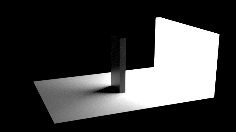
Before diving into the coding part of this project, take some time to review the newly added API functions. Try rendering some of the ambient occlusion tests in the scenes directory and make sure that you understand what's going on under the hood. You may find the API documentation page useful in this stage.
This project consists of the following parts:
- Adding support for area and environment map luminaires
- Implementing path tracer both with and without multiple importance sampling
- Creating a BSDF that describes a smooth dielectric material
- Testing your code to ensure that it works
2. Area and environment luminaires
A physically-based renderer must be able to manage the luminaires present in the scene in some form that permits efficient query and sample operations. Currently, the base code has no knowledge of luminaires whatsoever. Your task will be to devise an abstraction that is suitable for a path tracer and implement all necessary functionality including parsing, evaluation, and sample generation.
The details of the interface specification are completely up to you. In principle, a good way to get started is by creating a new top-level class named Luminaire that is similar in style to BSDF (though the information exchanged by the sampling and query functions must obviously be quite different).
You will create two different types of luminaires: an area light, which turns a triangle mesh into a spatially uniform Lambertian emitter, and an environment map, which loads a latitude-longitude OpenEXR lightprobe and uses it to simulate a illumination received from a distant environment. A set of lightprobes is available on Paul Debevec's website. That page also describes how to map between image coordinates and world-space directions. Since lightprobe images usually have extremely high dynamic ranges, a good importance sampling strategy is crucial.
Specfication:
To ensure that everyone ultimately supports the same scene description format, your code should be able to handle the XML input of the following style:
- <scene>
- <!-- Load a radiance-valued latitude/longitude bitmap from "grace.exr" -->
- <luminaire type="envmap">
- <string name="filename" value="grace.exr"/>
- <!-- Scale the radiance values by a factor of 2 -->
- <float name="scale" value="2"/>
- <!-- Rotate the environment map 30 degrees counter-clockwise around the Y-axis -->
- <transform name="toWorld">
- <rotate axis="0,1,0" value="30"/>
- </transform>
- </luminaire>
- <!-- Load a Wavefront OBJ file named "mesh.obj" -->
- <mesh type="obj">
- <string name="filename" value="mesh.obj"/>
- <!-- Turn the mesh into an area light source -->
- <luminaire type="area">
- <!-- Assign a uniform radiant emittance of 1 W/m2sr -->
- <color name="radiance" value="1,1,1"/>
- </luminaire>
- </mesh>
- <!-- ..... -->
- </scene>
The main thing to note is that there is at most a single environment map that is specified at the top level. There may be an arbitrary number of area lights, whose declarations are nested inside the associated mesh objects.
Some careful thought put into design (more mathematical design than laying out the class hierarchy) early in the process will pay off when you are implementing and testing. How are you going to sample luminaires during rendering? What interfaces should be provided to support the sampling of luminaires by the rendering code? (The BSDF interface is a good model here....) How can you test your luminaires in isolation to be sure they are working before you try to integrate them into the whole system?
3. Path tracing
In Nori, the different rendering techniques are collectively referred to as integrators, since they perform integration over a high-dimensional space. Begin by implementing a simple path tracer without multiple importance sampling as a new subclass of Integrator and associate it with the name "path" in the XML description language. This integrator should compute unbiased radiance estimates and use direct illumination sampling, as well as a russian roulette-based termination criterion. Once that is done, you will be able to render the supplied example scenes, though, as we saw in class, you can expect a lot of noise in scenes where one of the importance sampling schemes you are using does not perform well.
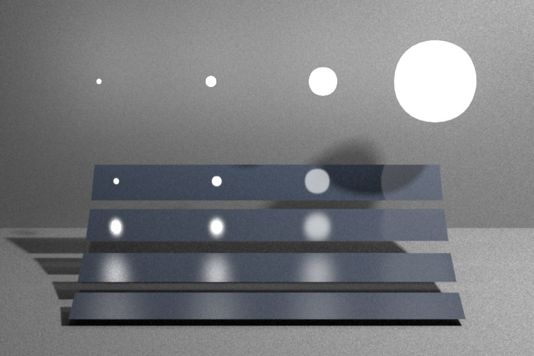
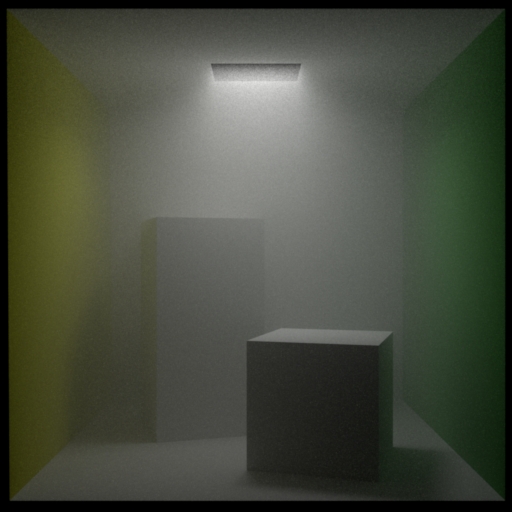
Following this, create a second integrator ("mipath") that now uses multiple importance sampling to combine luminaire and BSDF sampling strategies (using either the power or balance heuristic). Do you find that this improves the image quality compared to the original implementation? Does it always help? If everything works correctly, you should be able to reproduce the above rendering of Veach's multiple importance sampling test scene.
You may find it useful to also implement a renderer that uses only BSDF sampling. It will produce high variance when illumination is coming from luminaires that subtend a small region in direction space, but its correctness does not depend on the correctness of your luminaire sampling code, so it can be a useful debugging reference.
4. Dielectric material
Finally, extend Nori with an ideally smooth dielectric BSDF. It should support reflection and refraction using Fresnel's and Snell's laws, and it should conform to the following XML interface:
- <bsdf type="dielectric">
- <!-- Interior index of refraction -->
- <float name="intIOR" value="1.5"/>
- <!-- Exterior index of refraction -->
- <float name="extIOR" value="1"/>
- </bsdf>
5. Testing
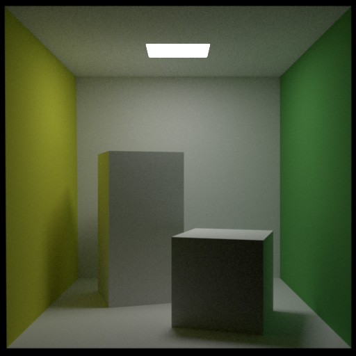
Please render the scenes included with the project, and ensure that you can match the following reference renderings (these were created using a large number of samples):
To view OpenEXR files, you can either use the exrdisplay command-line utility, Photoshop, or Edgar Velázquez-Armendáriz HDRI Tools. Please don't use the Mac OS Preview program— it can open EXR files but displays them incorrectly.
While checking the output visually is a good start, we know that the human eye is not the best measurement device. It's all too easy to implement a renderer with the required capabilities that appears to work but doesn't actually produce accurate results. Just as with the microfacet BRDF, you'll need to provide numerical test results showing that your program is working correctly.
The upgraded base code contains a modified t-test that is able to verify that a simple 1-pixel rendering converges to the right value. Run the renderer against the testcases in the scenes/tests-proj1 directory and report the output.
6. Extras (optional, not for credit)
Once you are done with the above, the following might be fun extensions:
- Modeling: Nori can handle a large range of scenes, as long as the contained meshes are specified using the Wavefront format. Create a new scene that highlights some of the features you have implemented.
- Sample generation: Currently, the render only provides a simple sample generator that produces a stream of statistically independent uniform variates. Implement stratified sampling, or use a Quasi-Monte Carlo (QMC) low-discrepancy number sequence to reduce the noise in the output renderings.
- χ2, v2.0: The importance sampling code of the environment map luminaire can be tricky to get right on the first attempt. Extend the χ2-test included in Nori so that you can use it to validate the directional sampling of this luminaire. This should be relatively straightforward and can potentially save a lot of time.
- Alternative reality theory: Buggy rendering algorithm implementations often produce strangely appealing yet completely non-physical renderings. Send us your craziest garbage result for potential addition to the gallery.
1. Introduction
At this point, you have a Monte Carlo path tracer at your command that is capable of producing realistic images of scenes designed using surfaces. In this assignment, you'll add support for homogeneous and heterogeneous participating media as discussed in class. This will extend the renderer's range to scenes including hazy atmospheres, subsurface scattering, plumes of steam or smoke, and other kinds of volumetric data (e.g. CT scans).
As before, we have released an upgrade to the Nori base code on github, which adds medium classes and some API code that you may find useful (but which you should feel free to change in any way). Please fetch and merge these changes into your current repository using git. Due to their size, the volume data files are not part of the repository on github. You can download them here: volume-data.zip.
For your reference we have also released sample solutions for project 1 on CMS.
Altogether, this project consists of the following parts:
- Implementing sampling and transmittance evaluation code for the two medium classes
- Adding the Henyey-Greenstein phase function model
- Extending the two path tracers with medium support
- Rendering the provided example scenes
- Testing your code to ensure that it works
2. Medium sampling
Production systems usually support rendering with arbitrary numbers of participating media that can be given complex shapes, e.g. by attaching them to surfaces in the scene. Implementing media at this level of generality is unfortunately very laborious. Here, we focus on the most basic case to simplify the project as much as possible: a single box-shaped medium. This time, all of the logic for constructing media from the scene description is already part of the framework code. For instance, the following scene description will instantiate a homogeneous medium and register it with the Scene class:
- <scene>
- <medium type="homogeneous">
- <!-- By default, the medium occupies the region [0,0,0]-[1,1,1]. Scale and rotate it: -->
- <transform name="toWorld">
- <scale value="5,5,5"/>
- <rotate axis="0,1,0" angle="45"/>
- </transform>
- <!-- Absorption and scattering coefficients -->
- <color name="sigmaA" value="0.01,0.01,0.01"/>
- <color name="sigmaS" value="1, 1, 1"/>
- <!-- Instantiate a Henyey-Greenstein phase function -->
- <phase type="hg">
- <!-- Configure as slightly forward-scattering -->
- <float name="g" value="0.5"/>
- </phase>
- </medium>
- ...
- </scene>
To account for medium scattering interactions, your renderer must be able to importance sample the integral form of the radiative transfer equation. To support direct illumination computations, it must futhermore be able to compute the transmittance between two world-space positions in the scene. Take a look at the existing homogeneous and heterogeneous media classes in src/homogeneous.cpp and src/heterogeneous.cpp and make sure that you understand what they do. Add support for the missing operations using sampling and evaluation techniques of your choice.
3. Phase functions
The framework already ships with an API and an implementation of a purely isotropic phase function. Add the Henyey-Greenstein model and verify it against the provided χ2-test in scenes/tests-proj2. You may find this PDF file useful.
4. Path tracers
In lecture, it was discussed how participating media can be incorporated into a surface-based path tracer. Add support to both your regular path tracer, and the variant with multiple importance sampling.
5. Example scenes
Reproduce the example scenes listed above. Below are references in OpenEXR format. Note that some of them use a higher number of samples compared to the distributed XML files.
- cbox-foggy.exr (4096 sample/pixel)
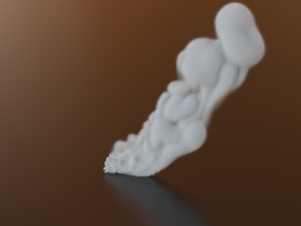
- steam.exr (1024 samples/pixel)
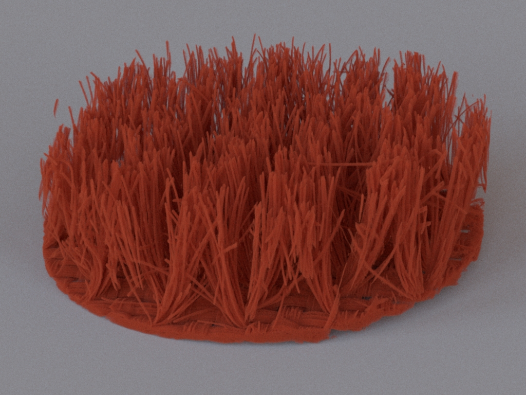
- velvet.exr (1024 samples/pixel)
- scatcube-mismatched.exr (1024 samples/pixel)
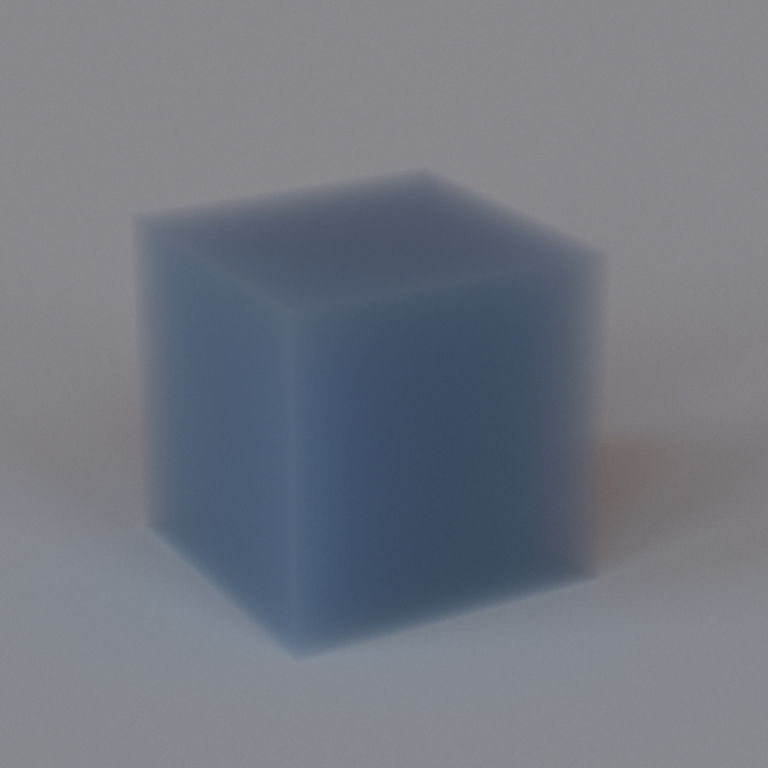
- scatcube-matched.exr (8192 samples/pixel)
You will notice that renderings of the index-mismatched homogeneous cube are much noisier when compared to the index-matched version (when done using the same number of samples). Why is this? The rendering also appears darker—what is the physical explanation of this effect?
Create a new scene based on the index-mismatched cube example, where the medium parameters now correspond to skim milk as listed in this paper. What do you observe when rendering this scene. How can you explain this in terms of your implemented medium sampling strategy?
6. Testing
It's all too easy to implement a renderer with the required capabilities that appears to work but doesn't actually produce accurate results. As before, have released a list of statistical testcases to ensure correctness. Please run the tests located in the scenes/tests-proj2 directory and report the results in your writeup (the detailed output is not necessary).
7. Extras (optional, not for credit)
Once you are done with the above, the following might be fun:
- Procedural clouds: Using the Perlin noise function, it is relatively straightforward to create procedural clouds. Implement and render a cloud or another procedural medium.
1. Introduction
Over the past few assignments, you've developed a fairly complete physics-based renderer based on the theory we discussed in class. The final project is much more open-ended: we ask that you either implement one of the following two graphics papers in Nori or that you propose a project of your own that is similar in size. Work on the final project will entail extracting the relevant information from the chosen paper, designing suitable abstractions, and changing the architecture of the codebase as you deem necessary.
For your final submission, produce an image showing off the capabilities of your renderer. You will have a chance to present your work in the final project session on May 11.
An short introduction of the two project suggestions is given below, but note that you can also propose a project of your own choosing. In this case, please discuss it with the course staff by April 24.
A Rapid Hierarchical Rendering Technique for Translucent Materials
While working on project 2, you will have noticed that certain simple scenes (e.g. the index-mismatched cube) require surprisingly long rendering times if noise-free results are desired. Because much scattering leads to smooth radiance distributions, intuition tells us that such scenes should be "easier" to render, which is fundamentally at odds with the observation.
In class, we discussed how diffusion theory can be used to approximate radiative transfer under certain conditions. The diffusion equation can be thought of as a Taylor expansion in the spherical domain, where only the first two expansion terms are kept. This draws upon the smoothness of the radiance distribution and ultimately leads to an equation that is considerably easier to solve.
A popular way of rendering many kinds of materials with subsurface scattering involves an approximate analytic solution of the diffusion equation under the assumption of half-space geometry (i.e. \mathbb{R}^3, where all points with z<0 are filled with a scattering medium, and the other side is completely empty). Obviously, that is a rather strong simplification when rendering anything other than a half-space. Yet, the resulting model generally produces reasonable answers, because diffusion happens at small scales where the local geometry starts to look like a half-space. It is a good example of a physics-motivated method that may not hold up to real-life measurements, but is good enough to produce visually plausible results.
Begin by reading the paper (PDF) by Jensen and Buhler. Feel free to get in touch with the course staff at this point if you have technical questions, or if you would like to get feedback on your approach before starting with the implementation. We expect that you incorporate the two passes discussed in Section 3 into Nori so that you can re-render some of our previous scenes using the proposed BSSRDF. The best way to do this is probably as follows:
- Extend Nori so that you can "attach" a BSSRDF to a mesh similar to how this is currently done for BSDFs
- Write code that generates uniformly distributed samples on the relevant meshes, and compute the irradiance at each one of them. We recommand that you do not implement Turk's point repulsion algorithm and use the much simpler function Mesh::samplePosition() instead. The samples won't be as nicely distributed, which essentially just means that you will need more of them. Note that you will need to make small changes to the architecture so that this pre-processing phase is executed before the main rendering task.
- Implement the discussed octree traversal, and compute the scattered subsurface radiance using Equation 8.
A Simple and Robust Mutation Strategy for the Metropolis Light Transport Algorithm
The two path tracers in Nori provide a clean and general-purpose approach for rendering images. For certain types of input, they unfortunately require excessively large number of samples per pixel (and hence, a very long time). In designing these algorithms, we followed the Monte Carlo integration mantra of "\langle g\rangle=f/p" and chose sample distributions p to be nearly proportional to f whenever possible. But there are limits to what can be accomplished analytically. In particular there are many terms that are not considered by the sampling procedure, and these are what cause the aggregate importance weight \langle g\rangle to be far from constant.
In an abstract sense, we can think of a path tracer as a function that consumes random numbers and computes a value (i.e. an estimator for radiance) based on this input. The computational aspect is completely deterministic—all of the randomness stems from the input numbers. Suppose this function is called f(\xi_1, \xi_2, \ldots) where \xi_i denoted the ith random number. By drawing many samples and averaging the results of the path tracer, we essentially compute a high-dimensional integral of a "hypercube" of random numbers g=\int_0^1 \int_0^1 \cdots \ f(\xi_1,\xi_2,\ldots) \, \mathrm{d}\xi_1\, \mathrm{d}\xi_2\ldots The problem of stochastic path tracing is that it uniformly evaluates points in this space. If there is some small region in this hypercube where f takes on high values, it may only receive a few samples, and that is the reason for the noise issues you may have encountered when rendering the example scenes.
To build a better path tracing algorithm, it is desirable that it will spend more time in places where f is large. Yet, doing so is tricky without compromising the correctness of the algorithm. The above paper presents a clean approach that leads to an unbiased method. To accomplish this, it builds upon the Metropolis-Hastings algorithm. The basic idea is that we can keep track of the ``random numbers'' (\xi_1,\xi_2,\ldots) that are passed to the function f. In each iteration, these numbers are slightly perturbed, yielding (\xi_1+\varepsilon_1,\xi_2+\varepsilon_2,\ldots). We then look at the ratio r=\frac{f(\mathbf{\xi}+\mathbf{\varepsilon})}{ f(\mathbf{\xi})} If r>1, the function value increased, and we keep the perturbed "random numbers". Otherwise, we revert to the unperturbed values with probability 1-r. When doing this repeatedly, it can be shown that the sample density of this iteration will be proportional to f.
Begin by reading the paper (PDF) by Kelemen et al. Feel free to get in touch with the course staff at this point if you have technical questions, or if you would like to get feedback on your approach. The best way to incorporate this method into Nori is probably as follows:
- Implement a new subclass of Sampler that implements the logic needed to keep track of the fake random numbers. This part should be relatively straightforward, since the paper provides C-code.
- Implement an alternative rendering loop that contains the Metroplis-Hastings iteration. Note that it should operate on an entire image at once— the tile-based processing that is currently being used by the path tracers is incompatible with this technique.
- This algorithm only renders the image up to a multiplicative scale factor. To recover this constant, a brief path-tracing pre-process pass will be needed.
- Combine the path tracer with the new sampler and rendering loop
Gallery
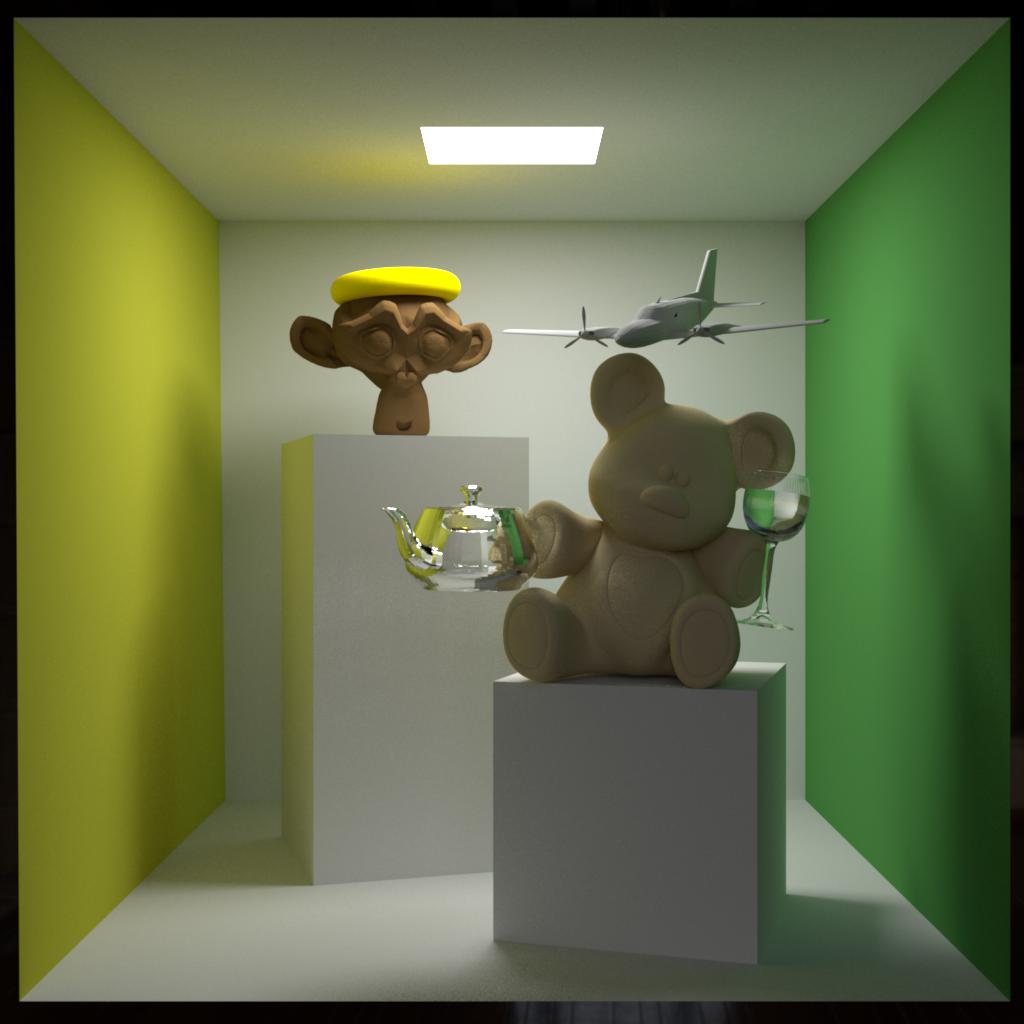
Awesome box
A beefed-up Cornell box! (by Brian Phlipot and Sean Ryan)
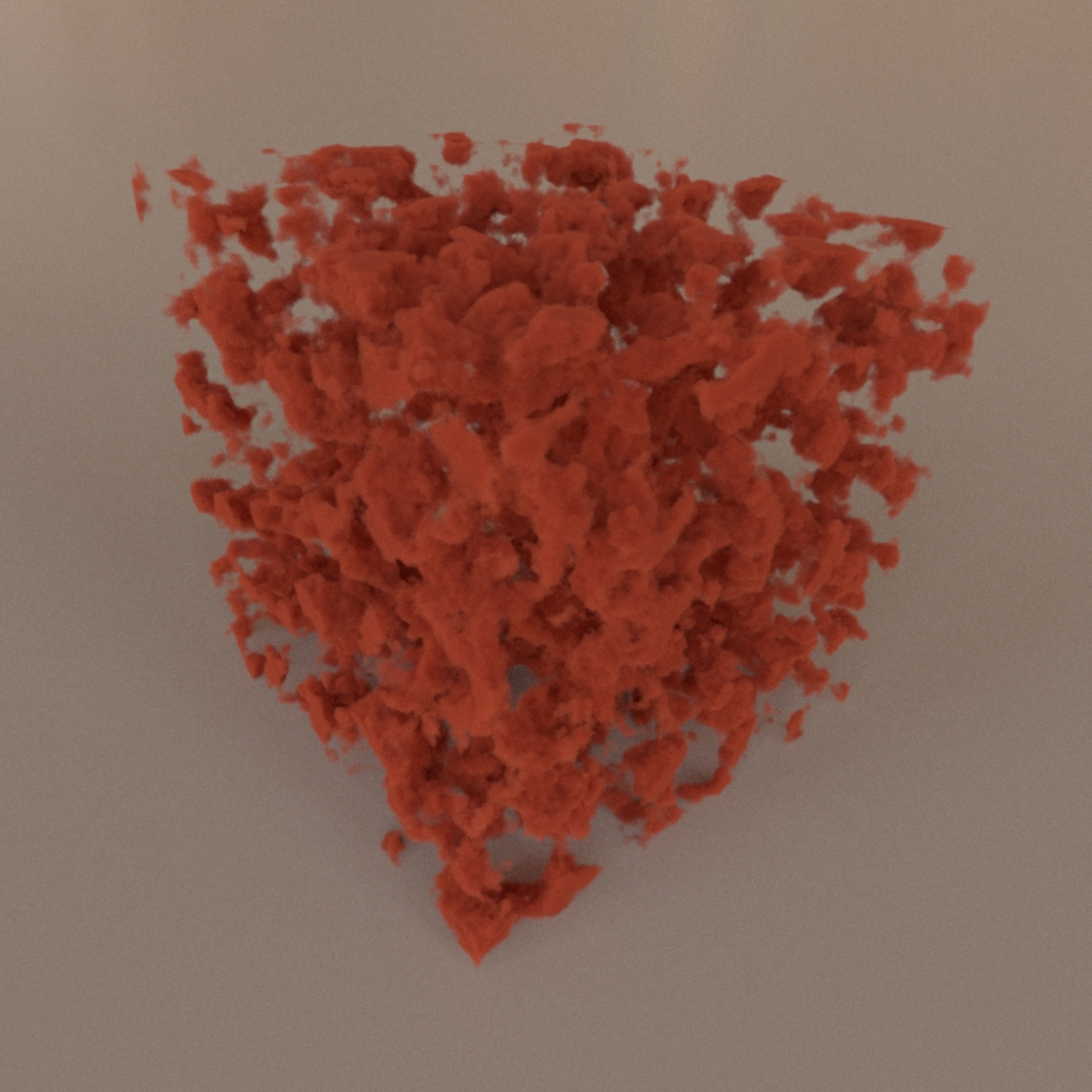
Spongy noise
Procedurally generated perlin noise sponge (by Sean Bell, Pramook Khungurn, and Timothy Langlois)
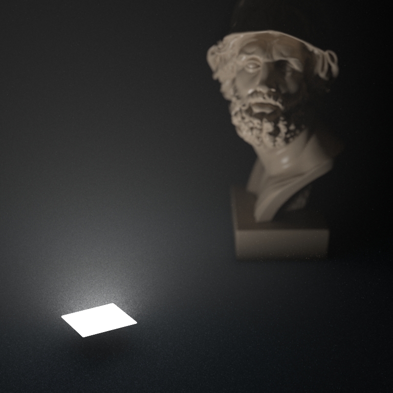
Ajax museum exhibit
Illuminated ajax bust in a dusty atmosphere (by Zhiyuan Teo)

Lucy in the sky without diamonds
Lucy on a microfacet floor, surrounded by the mists of a Perlin noise-based heterogeneous medium and lit with Debevec's Pisa environment map (by Asher Dunn and Nicolas Savva)
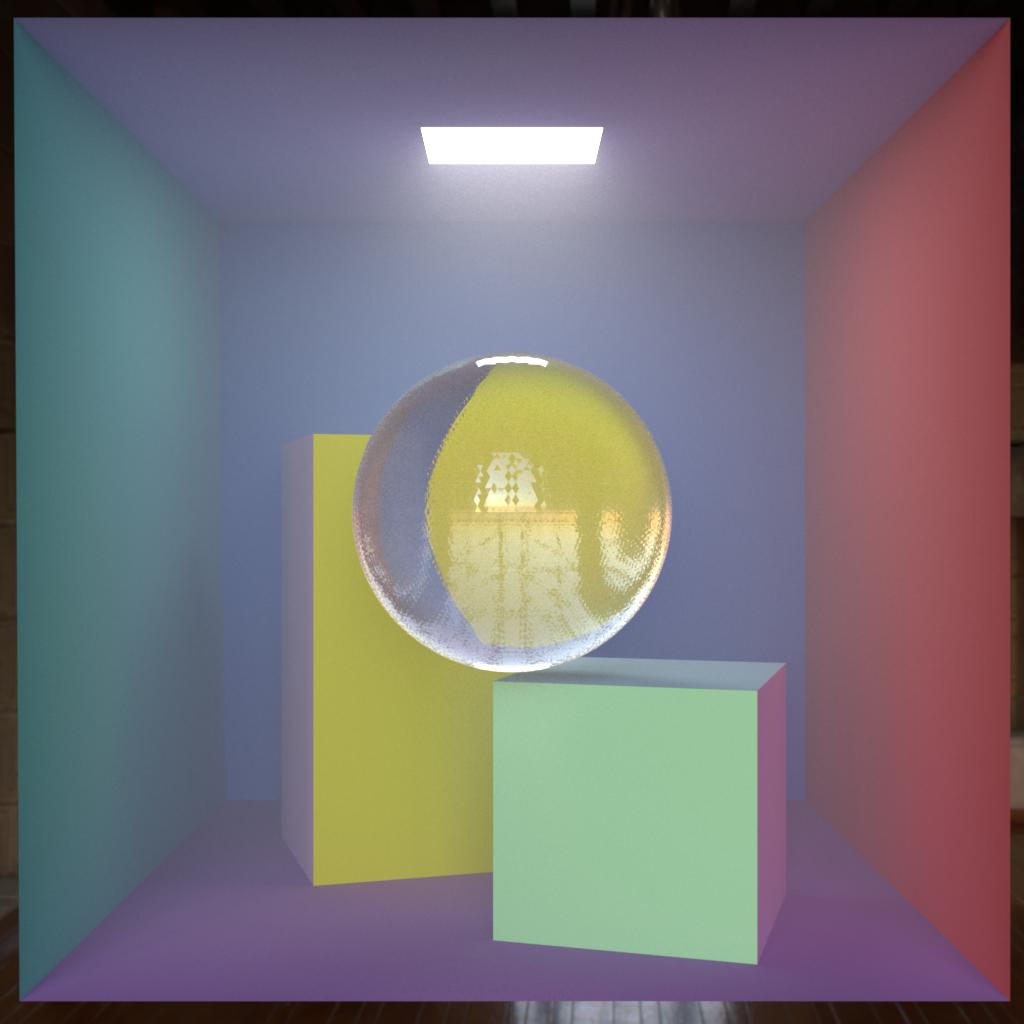
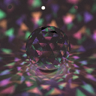
Colorful
A misty Cornell box with environment map lighting and a dielectric sphere (By Brian Phlipot and Sean Ryan)

Energy!
A phase function "normalized" to 2 instead of 1 (by Asher Dunn and Nicolas Savva)

Dragon box
A glass Stanford dragon in a Cornell Box (by Sunling Yan, Daniel Joerimann and Jordan Robinson)
Final Project Gallery
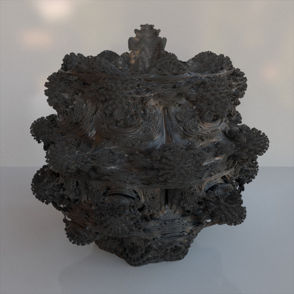
Mandelbulb fractal
Rendered by marching through a fractal distance field in spherical coordinates, with environment map lighting (by Sean Bell, Pramook Khungurn, and Timothy Langlois)
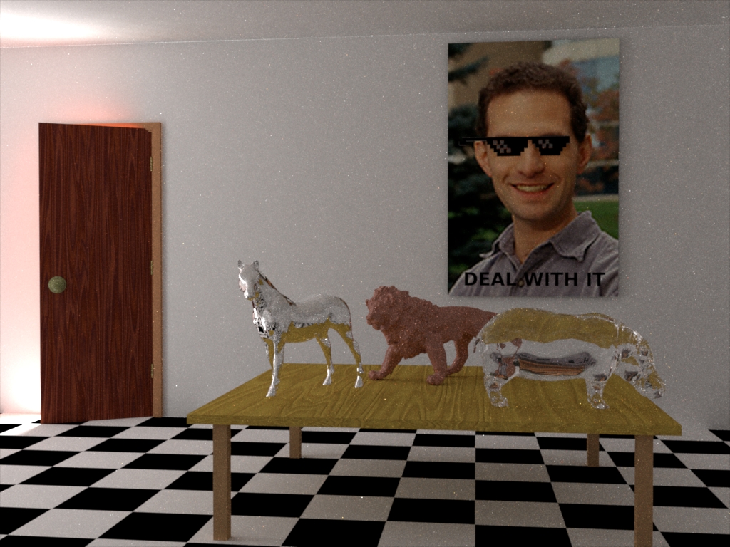
Ajar
All lighting is indirect from a door that is slightly ajar (inspired by Eric Veach's MLT scene, by Sean Bell, Pramook Khungurn, and Timothy Langlois)
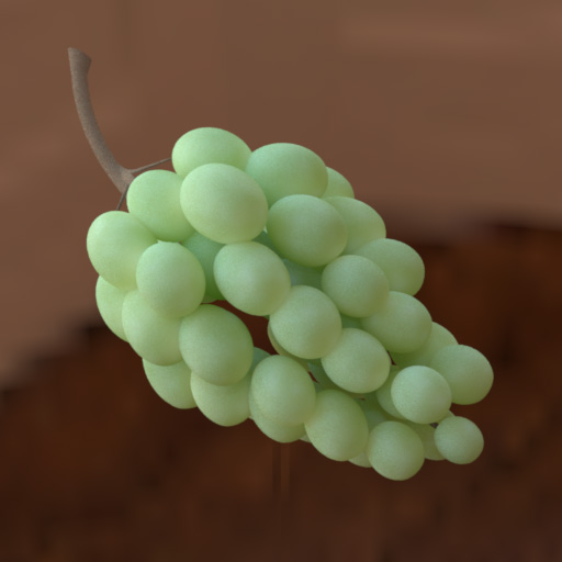
Grapes
BSSRDF grapes lit by an environment map (by Brian Phlipot, Sean Ryan, Asher Dunn, and Nicolas Savva)
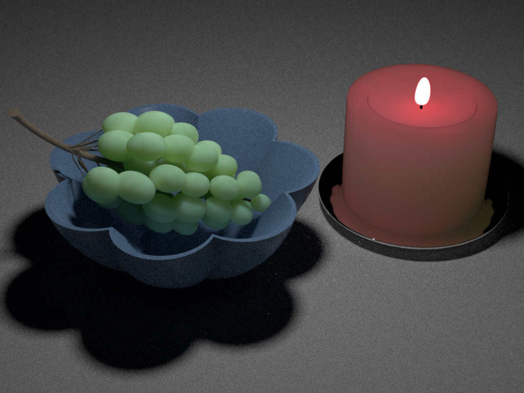
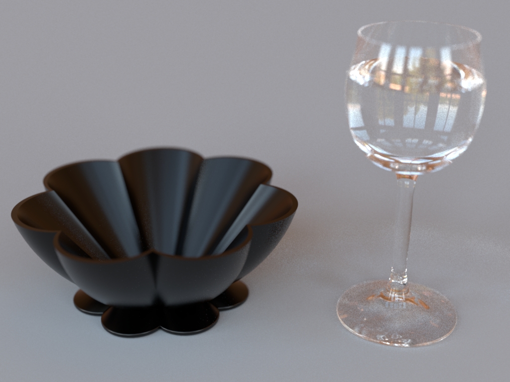
Grapes
The same grapes as before—now placed into a microfacet bowl and lit by a spherical light and a translucent candle. (by Brian Phlipot, Sean Ryan, Asher Dunn, and Nicolas Savva)
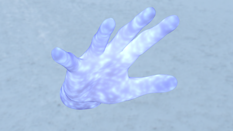
Ethereal
A subsurface scattering hand rendered using settings for 'blueish' skin (by Devansh Gupta and Jin Hyuk Cho)

Ant wars
A complex scene involving caustics, rendered using Kelemen-style MLT (by Kevin Matzen, Zhiyuan Teo, and Chun-Po Wang)
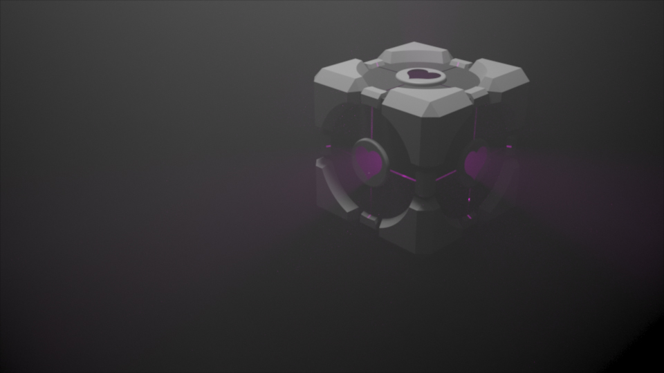
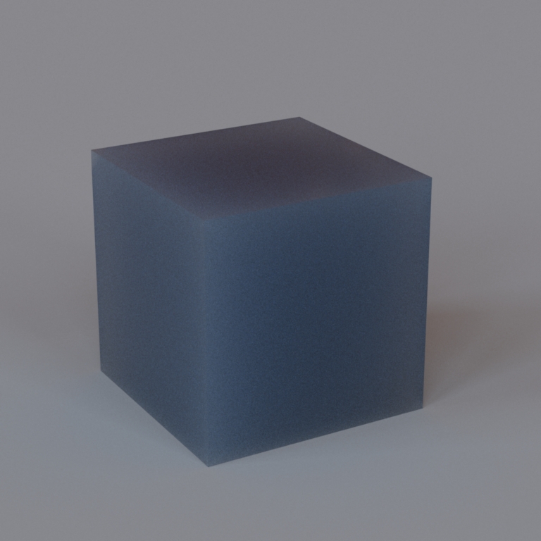
Companion Cube
A radiant companion cube in a misty atmosphere, rendered using Kelemen-style MLT (by Kevin Matzen, Zhiyuan Teo, and Chun-Po Wang)
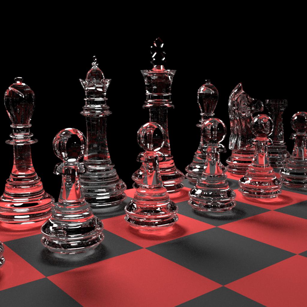
Chess
A complex refractive chess scene, rendered using Kelemen-style MLT (by Jeff Ames, Alessandro Farsi and David Thomason)
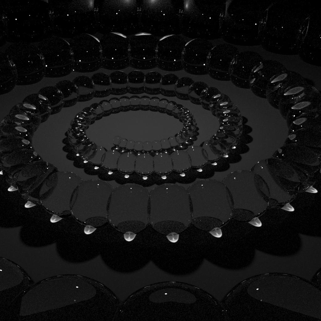
Caustic spiral
A spiral of spheres with caustics, rendered using Kelemen-style MLT (by Jeff Ames, Alessandro Farsi and David Thomason)