Assignment 2. Pipeline
Table of Contents
The Pipeline assignment is a 3-week project with weekly checkpoints. Work by yourself or with a partner, as always.
1 The Basics
This week is mainly about putting together the machinery to supply a scene and to render it using OpenGL with the desired shader programs, which will be the basis for implementing fancier shading methods.
1.1 Take a look at GLWrap/ and Demo/.
We are providing a simple library called GLWrap to abstract some of
the features of OpenGL, and to help keep track of the OpenGL objects you
create by associating each one with a C++ object. The lifetimes of these
paired objects are matched: the OpenGL resource is created at the time
that the C++ object is created, and when the C++ object is destroyed,
the OpenGL resource is released. The wrapper classes are designed to
provide fairly direct access to the OpenGL API for manipulating the
wrapped objects, but they all also have an id() method that
gives you the OpenGL handle for the wrapped object so you can make any
calls you need directly to the OpenGL API.
Also, there is a new addition to the Demo directory called TetraApp that illustrates several things that are useful in this assignment:
- Creating an instance of
GLWrap::Programthat compiles and links a set of shaders. - Creating an instance of
GLWrap::Meshand populating it with a vertex position buffer and an index buffer. - Drawing the mesh by providing the necessary uniforms to the program
and calling
Mesh.drawElements. - Using explicitly specified numerical locations to match attribute buffers to shader inputs.
- Using the
CameraandCameraControllerclasses in RTUtil to provide camera control, including overriding the Nanogui event handlers and passing the events to the camera controller.
You run this app by providing the command line argument string
“Tetra” to the Demo executable: ./Demo Tetra. (Or pass the
argument using the settings in your IDE.)
1.2 Make a new app that draws a hard-coded mesh.
You can go ahead and use the same fork as the ray tracing assignment for developing your solution. Be sure to fetch all changes from upstream (i.e. from our starter code repository). This way fixes to the libraries can easily be merged into your work, and additional updates can be merged in without disturbing your process.
In your working copy, create another Nanogui app, in the same way you
did for the ray tracer. I put mine in a directory called
Pipeline/. This time you can inherit directly from
nanogui::Screen since you don’t need the image display
provided by RTUtil::ImgGUI. Populate your class with the
contents of the Tetra demo. You’ll need to add an entry for your new app
in CMakeLists.txt. Make sure you can compile a working app;
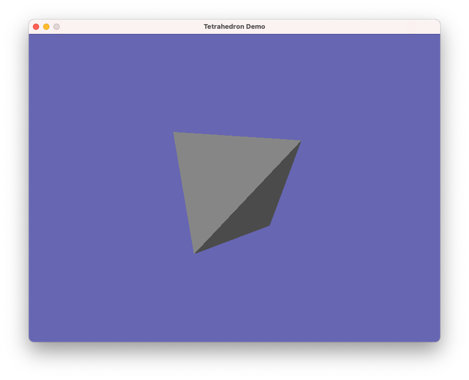
you should see a tetrahedron
that you can spin around with the mouse.
You’ll note that the Tetra demo uses a shader program composed of
three shaders read from resources/shaders:
min.vs: a vertex shader that outputs vertex positions in eye space as well as the position in NDC.flat.gs: a geometry shader that associates each triangle’s geometric eye-space normal with all of its vertices.lambert.fs: a fragment shader that computes Lambertian shading in eye space.
This is a nice little setup for getting up and running with minimum input, but it’s worth noting that the flat shading geometry shader is not what you will ultimately want. In my solution I kept it around as a debugging tool for rendering when something is wrong with the normals. But I’ll say it again: don’t get confused by this; it is not the normal way to do things! You normally pass normals as vertex data, which we will do soon enough.
1.3 Load and draw a single mesh
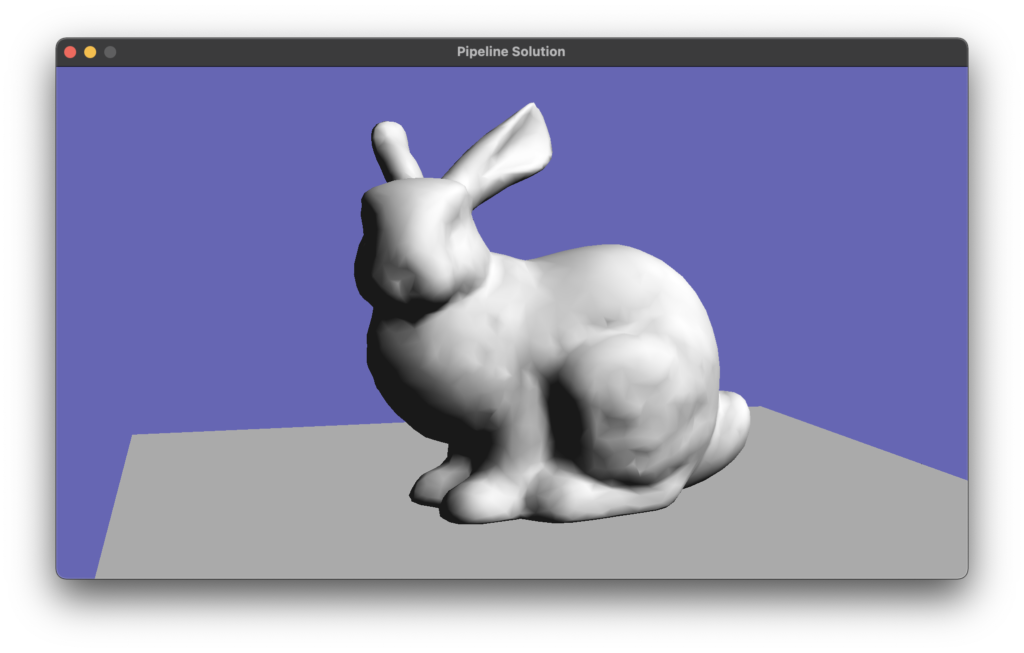
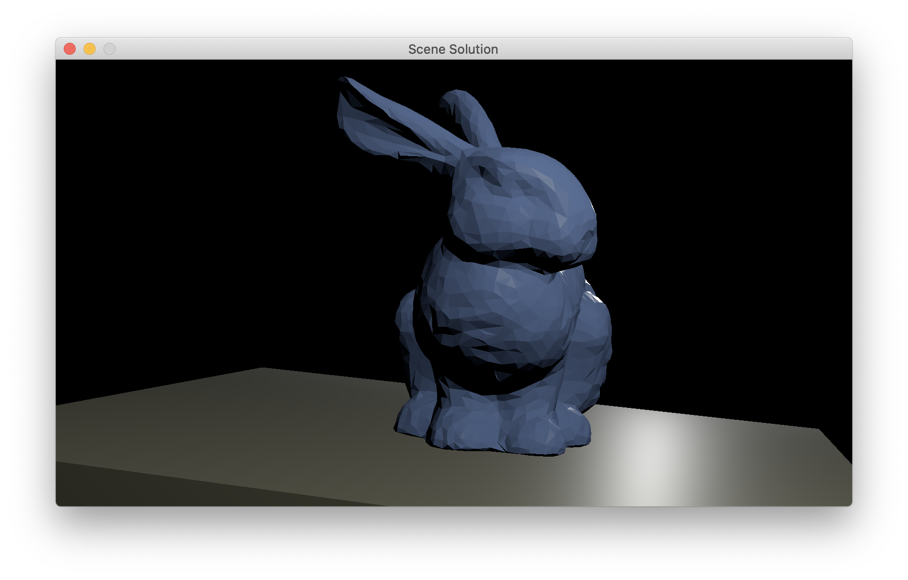
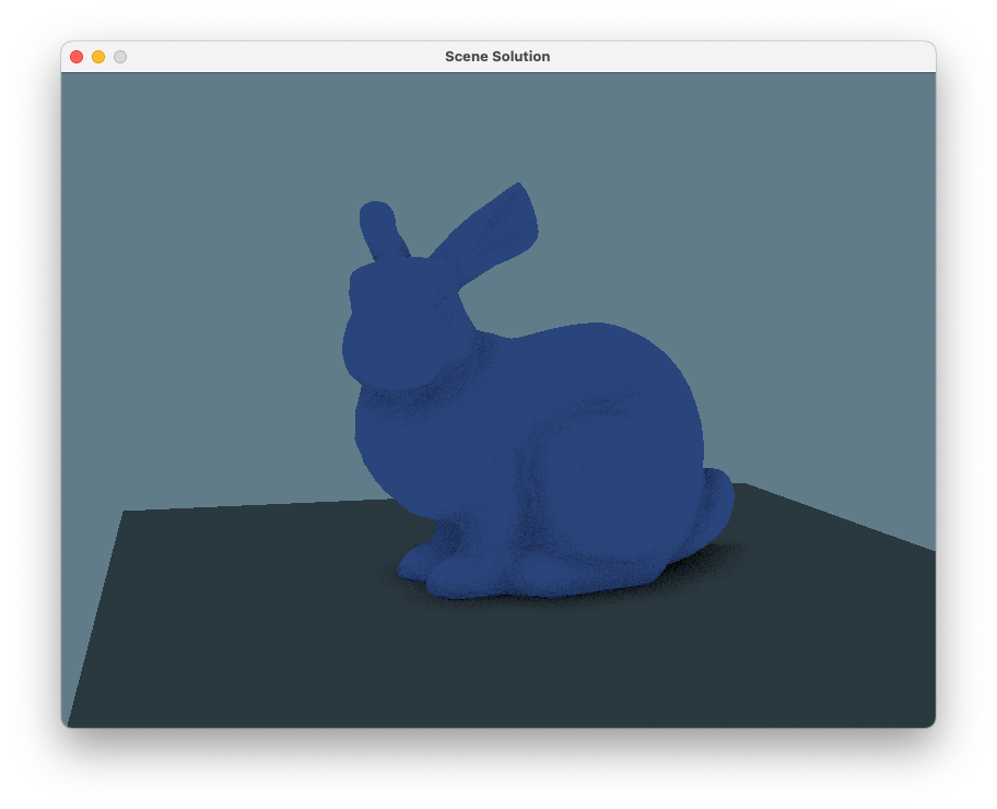
In this step we’ll get to the point where we can draw a single OBJ mesh, still using a fixed camera. To use the bunny as a test, you can instantiate the camera with the following parameters:
PerspectiveCamera(
    glm::vec3(6,2,10), // eye
    glm::vec3(0,0,0), // target
    glm::vec3(0,1,0), // up
    windowWidth / (float) windowHeight, // aspect
    0.1, 50.0, // near, far
    15.0 * M_PI/180 // fov
)
and it will give you a reasonable view of the bunny.obj test mesh.
Making liberal re-use of your scene loading code from the previous assignment, write a function that reads in a scene via assimp, loading the scene hierarchy into a node hierarchy of your own devising. Our node hierarchy consists of two classes:
Node, which contains a transformation, a list of mesh indices, a list of pointers to childNodes, and a pointer to a parentNode.Scene, which contains a list of meshes, a camera, the same lists of materials and lights as in the previous assignment, and a pointer to the root node.
Then modify your program so that instead of drawing the hardcoded mesh it just draws the first mesh in the scene. For now don’t worry about transformations, and just test with OBJ files, which have all the meshes in world space.
Once you have this set up, you should be able to draw the bunny with an intial view matching this reference, and then spin it around with the mouse. (The camera controller that the Tetra demo uses is not the greatest; you will find your program is more fun to use if you improve it.)
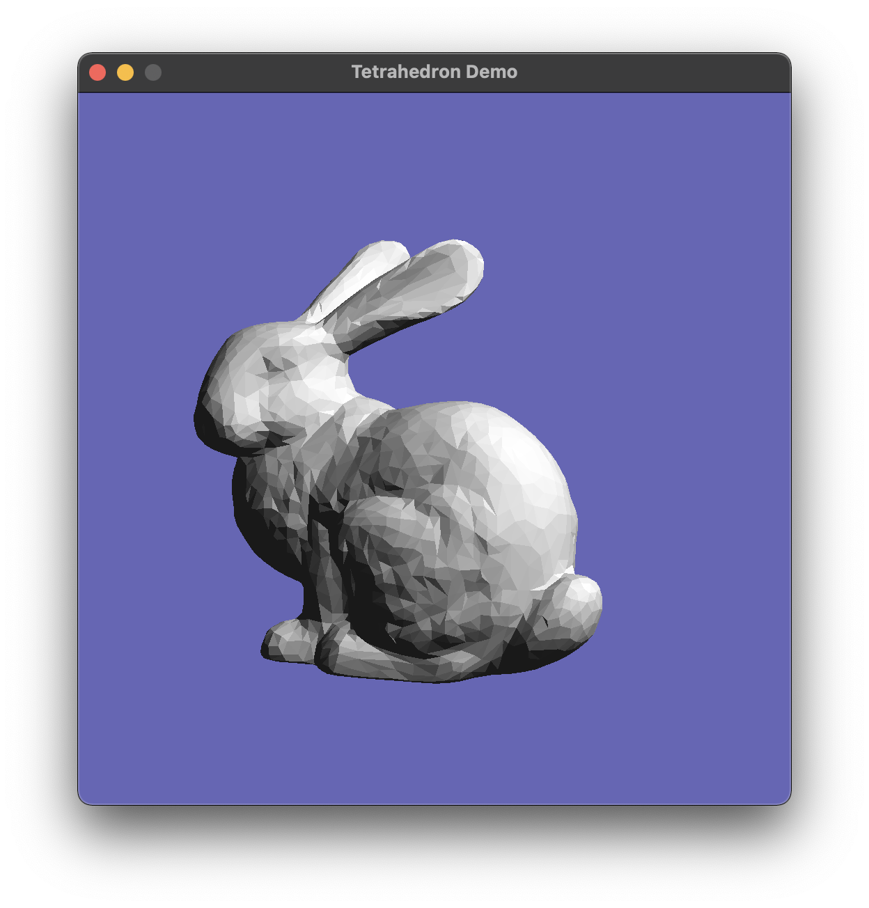
When you are designing your scene loading logic, one constraint to be
aware of is that you cannot make any OpenGL calls until after the
nanogui::Screen constructor has run, because that is when
nanogui creates the OpenGL context. This means that, if you
follow the same pattern as TetraApp and subclass
nanogui::Screen, the subclass constructor is the earliest
you can start building GLWrap::Mesh instances, etc.
1.4 Draw scenes with transforms and cameras.
Now fix up your program so that it can properly load and display a
scene with many objects and view it with the camera provided in the
scene. This step is simple but requires a little care, but relying on
your experience (and code) from the first assignment, you should not
need to do much that is really new. If you want to take advantage of
RTUtil::Camera and its camera controller, you’ll need to
change your camera-loading logic so that it creates an instance of
RTUtil::PerspectiveCamera from the parameters stored in the
aiCamera.
One wrinkle is that the provided camera keeps track of its state in
terms of an eye point and a target point, but aiCamera has
an eye point and a view direction (called confusingly
lookAt). For good camera control the target point (about
which the camera will rotate when orbiting) needs to be placed at a
reasonable location in the scene, and something that works well for our
scenes is to put it near the origin. Specifically, what we did was to
place the target point at the closest point to the origin along the
camera’s center viewing ray (the ray defined by the eye point and the
view direction).
The biggest difference between the two assignments is that in the ray
tracer we applied the transformations to the meshes and then left them
behind: the ray tracing engine expected all the meshes to be in world
coordinates. In this assignment we could potentially do the same thing,
but the conventional approach (important for scenes that might be edited
or animated) is to keep the meshes in the same coordinates they come in
(object space) and apply the transformations at the time of drawing. To
implement this, you only need to keep the transformations from the
Assimp model in your own node hierarchy, and modify your scene traversal
so that it accumulates the transformation needed for drawing, and copies
that transformation into the appropriate shader program uniform. (A
prime opportunity for mistakes is getting the transforms in the wrong
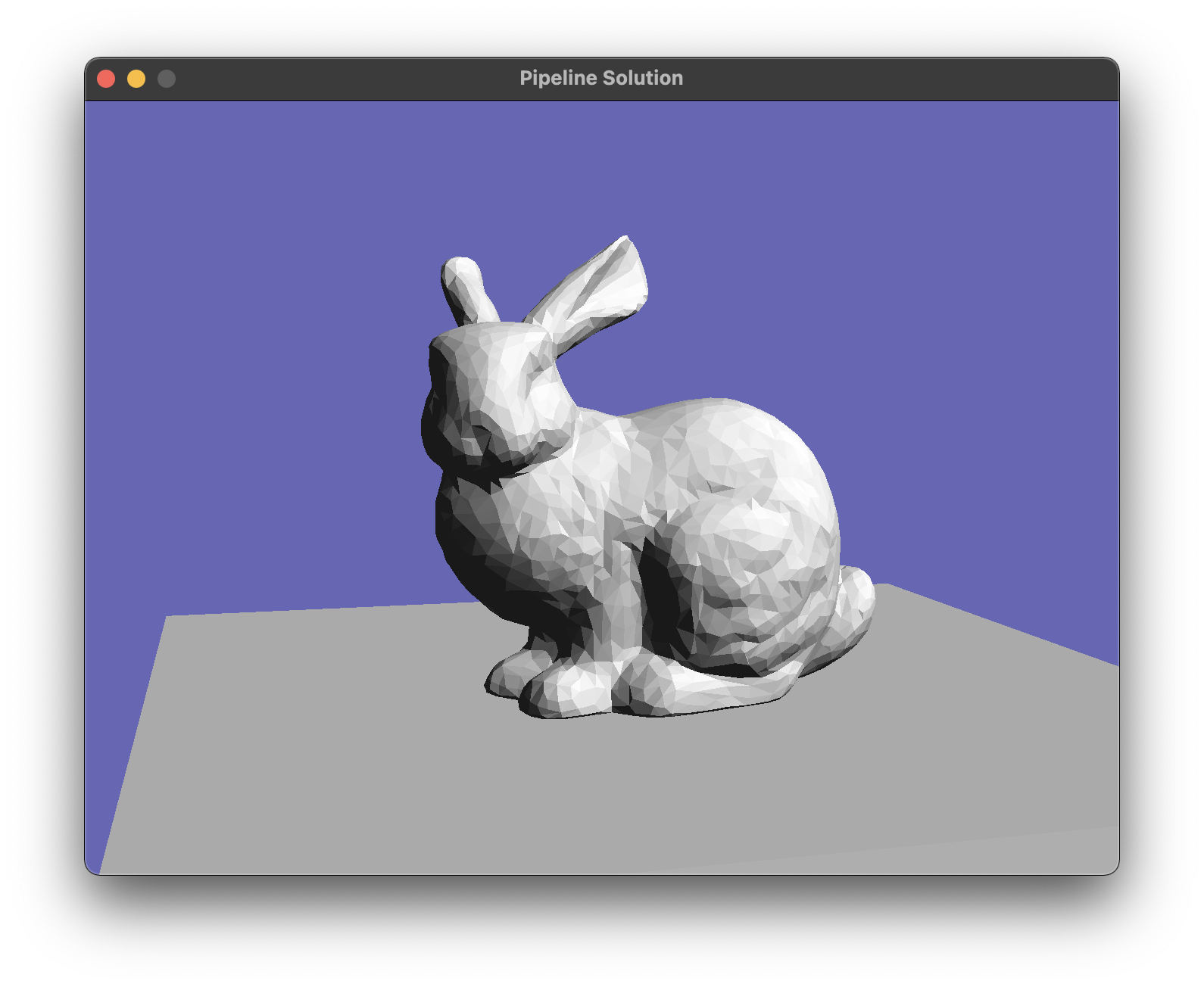
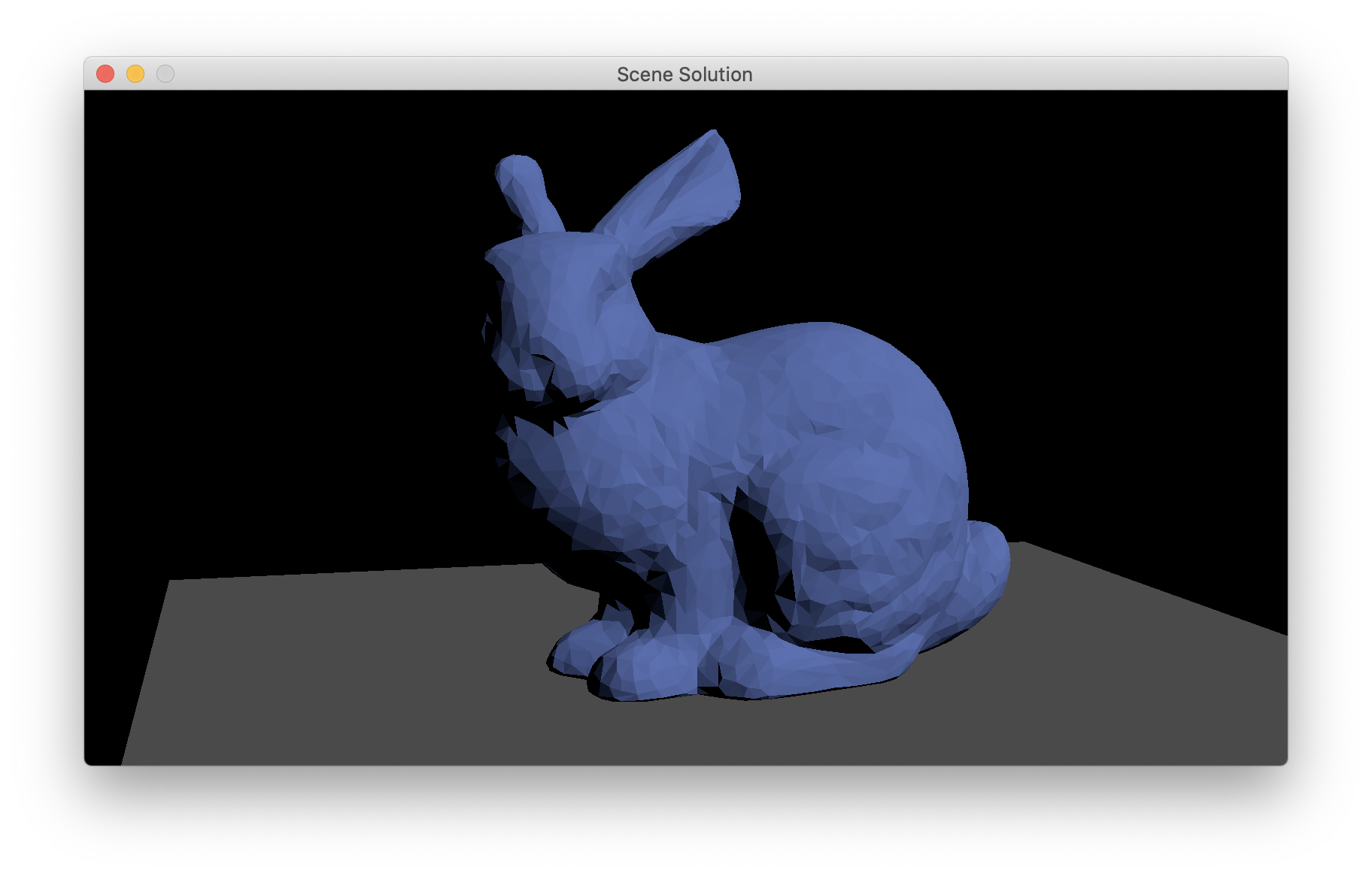
order.) Once this is done you should be able to load
bunnyscene.glb and see the bunny and the floor.
Here is a reference for
bunnyscene.glb with the transformations used but still with
the default camera.
To complete this step, change your code so that it uses the scene camera, if it exists, in place of the default hard-coded one. (To maintain the ability to test with single OBJ meshes, it’s a good idea to add logic that supplies a default camera if the scene has no cameras.) It’s nice to also set the size of the window to match the aspect ratio of the camera (and if you don’t, you need to update the camera’s aspect ratio to match the window). That’s really about it! Once this is done you should get the familiar matching view of the bunny scene.
Try out some of the other scenes, too! One change you’ll notice in
this assignment is that I have given up on keeping all faces
front-facing. This is partly so we can use models like the tree that
have single-layer geometry, and partly out of laziness because many
models that are fun to use have inconsistent face orientation and it is
a lot of fuss to repair them. The main cost is that we cannot use
back-face culling as an optimization. I find the simplest way to do this
is to check the boolean GLSL fragment-shader builtin
gl_FrontFacing, and reverse the normal vector for
back-facing fragments.
1.5 Use the vertex normals that come with your mesh.
To get the right rendering quality we should use vertex normals that
come with our models. This is made simpler if we can assume that all
meshes come with normals. Assimp can arrange for this; it provides a
number of preprocessing options documented here,
and the aiProcess_GenNormals flag will get it to compute
flat-shading normals. (You can pass these flags in the second argument
of Assimp::Importer::ReadFile.)
Using the normals involves a few small changes:
- when you set the positions as a mesh attribute, also do the same with the normals but give it a different index (I used 1).
- declare an attribute in your vertex shader with
layout(location = 1)so that it will pick up that attribute. - make a vertex shader that passes that attribute to the the vNormal input of the Lambert fragment shader.
- build a program without the
flat.gsgeometry shader.
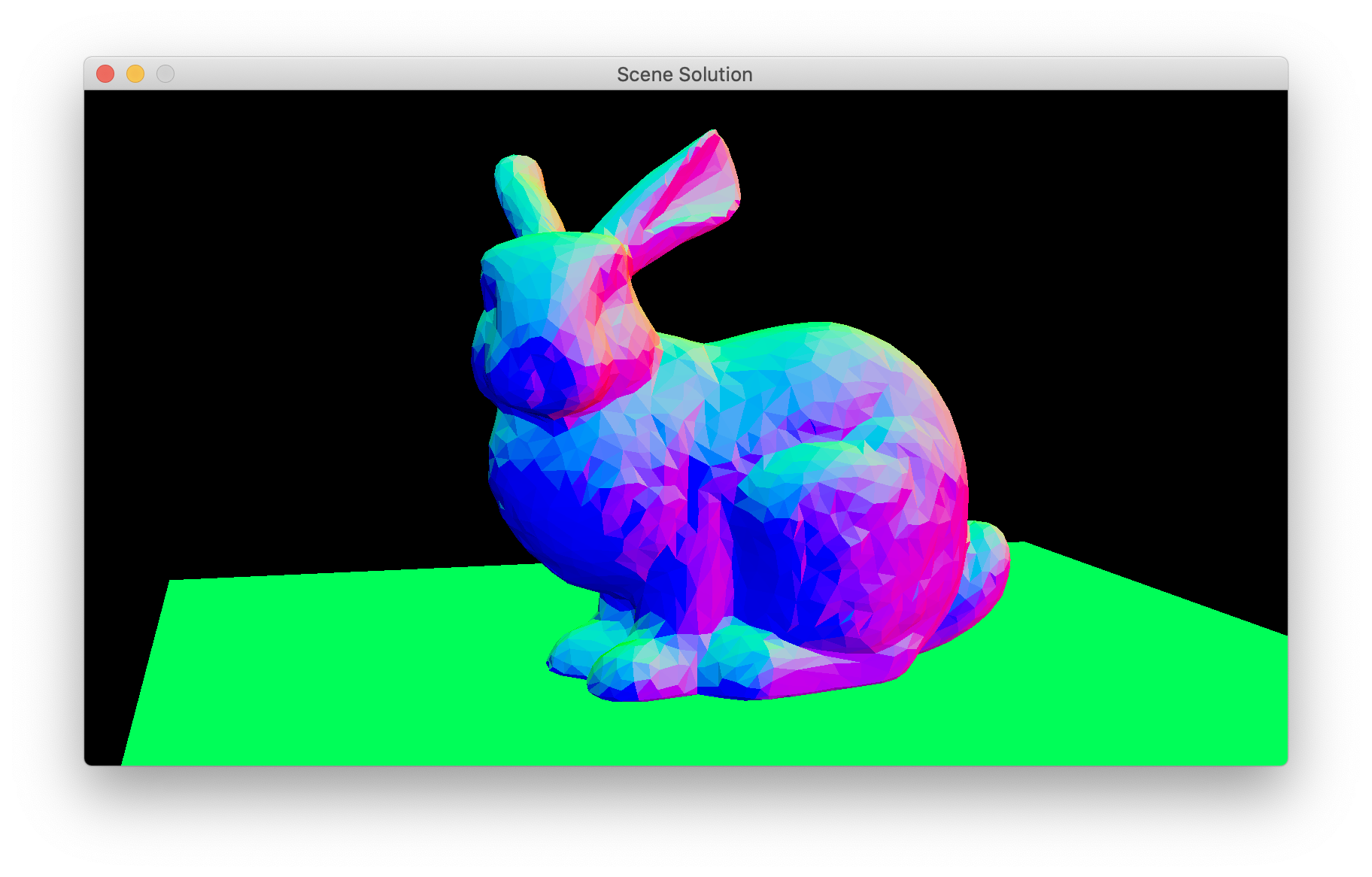
Then you should see smooth shading if you render a mesh with vertex normals (smoothbunny.glb), and flat shading if you render a mesh without normals (bunnyscene.glb). You might like to keep the flat shading shader around; I made the key “f” toggle a flag that chooses between these two shading modes.
I also found it useful to implement a feature to draw the normals, just for debugging. I did this with a geometry shader that takes in triangles and outputs line strips, and turns each triangle into three two-vertex line strips, which I then draw using a constant-color fragment shader.
1.6 Deal with materials and lights
To get things looking correct we of course need materials and lights. As with the previous assignment we’ll have just one material, a microfacet material, and materials are specified in the same way as before. So repurpose the same code you wrote earlier to set up your materials in your scene data structures, with one material associated to each mesh.
Then generalize the lambert.fs shader so that it
computes shading from a single point light using the Microfacet BRDF.
This means adding uniforms for the material parameters and light source
info, and implementing the shading calculations in the shader code.
Eventually we will deal with arbitrary numbers of lights, but for now
just support one, and use the properties of the first point light in the
scene.
To save you coding up and debugging it, we have included a GLSL
function to evaluate the microfacet BRDF in microfacet.fs.
I expect you’ll go on using the nori::BSDF class to
represent materials; you can get the Microfacet model parameters by
casting to Microfacet and calling the functions
alpha(), eta(), and
diffuseReflectance() to access the parameters. (Don’t
forget about the constant factor in converting from diffuse reflectance
to BRDF value.) Note that the C++ and GLSL implementations will not
match exactly because one uses the Beckmann distribution and one uses
the GGX distribution—but the size and brightness of highlights will be
very similar.
It is convenient to retain the ability to render bare OBJ meshes by providing a reasonable default light when there are no lights in the input.
Note that the code you wrote earlier will have computed light source parameters in world space; depending on where you decide to compute shading (in eye space or world space) you might need to transform the light before passing its position to the shader.
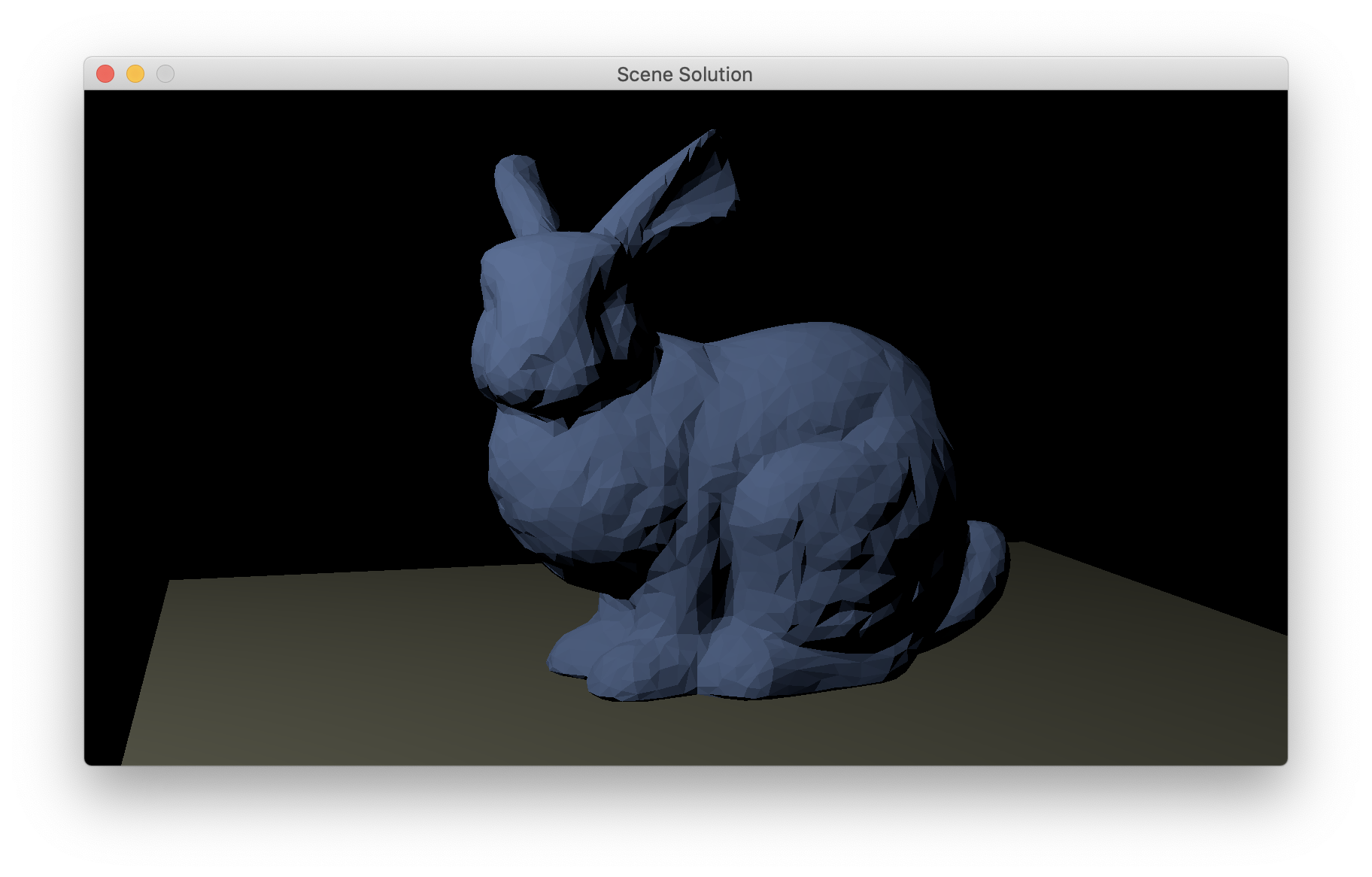
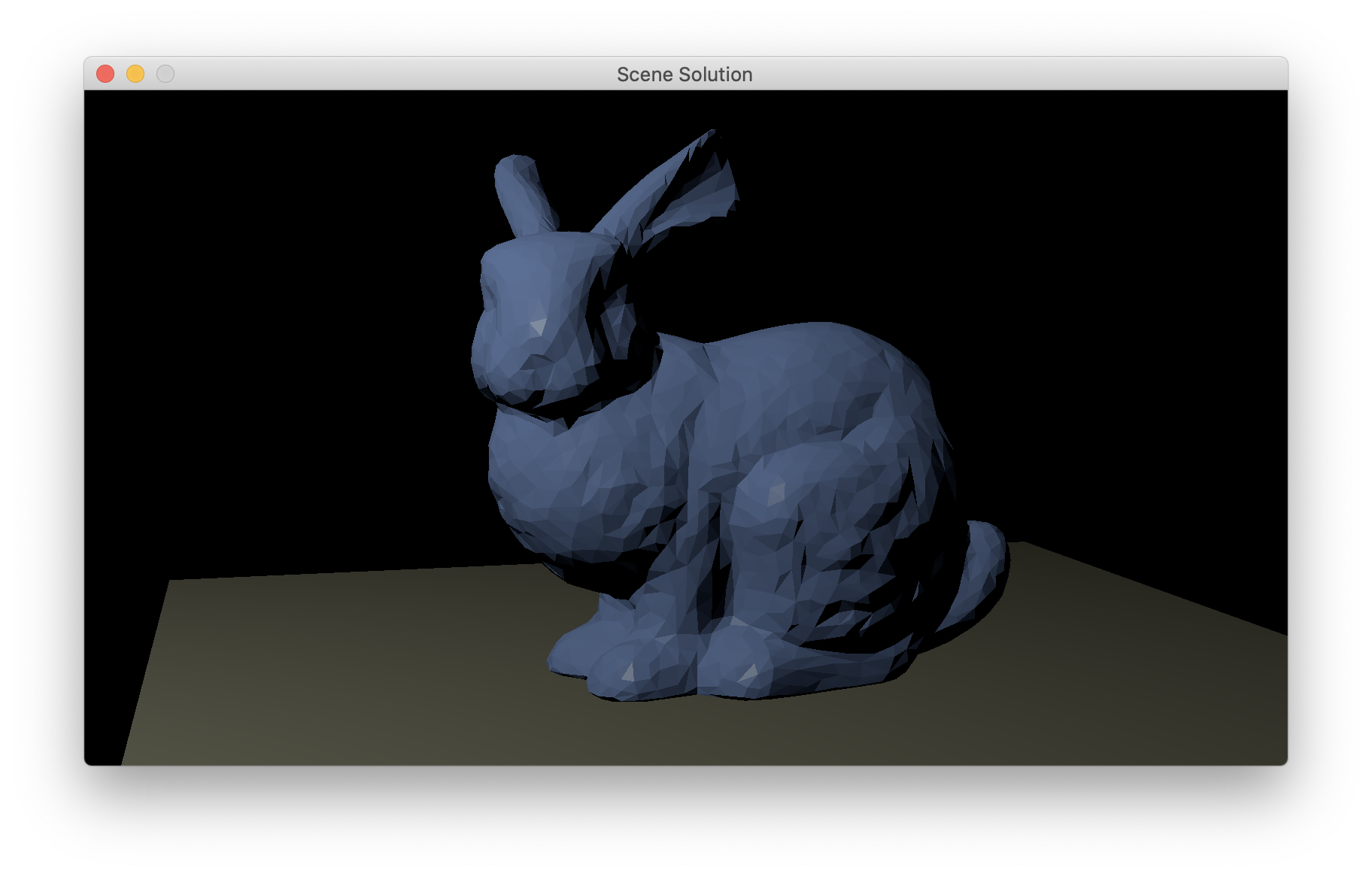
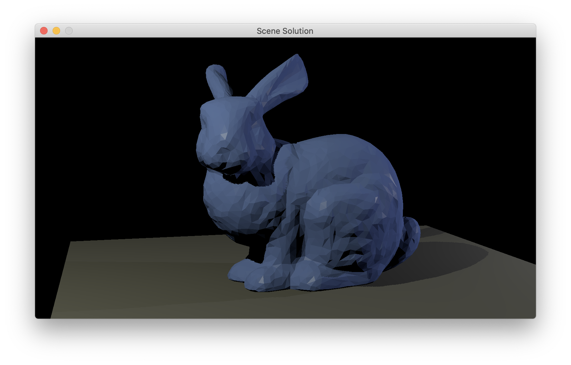
When you are done with this you will have the ability to render images that closely match the output of the ray tracer for a scene with a single point light, except that they don’t have shadows (yet). (Don’t forget about gamma correction!) References here (smoothbunny.glb) and here (bunnyscene.glb).
This is the checkpoint for Week 1. You should have this much working on Mar 17 and hand in a very short video showing it off.
2 Deferred shading and shadows
This week is about shifting to deferred shading, and drawing arbitrary numbers of lights with shadows. Just as a brief recap, the idea of deferred shading is to render in two passes: in the first pass, you draw the geometry as you normally would, but the fragment shader doesn’t actually do any calculations; it just writes the values required for shading computations into a geometry buffer or G-buffer. Then on the second pass, no geometry is needed; a more complex fragment shader simply runs once at each pixel, which reads from the G-buffer, does the required lighting computations, and writes the result into an output buffer. With deferred shading there is no need to limit the number of lights supported, since they can be rendered one at a time.
We’ll render shadows using shadow maps; recall that the idea of shadow maps is to use a depth buffer rendered from a virtual camera located at the light position to determine whether individual fragments to be shaded are on the closest surface to the light (illuminated) or behind that closest surface (shadowed).
Be sure to read through the week, or at least look at the list of pitfalls at the end, before you start coding in earnest.
2.1 Draw to a framebuffer
To do multi-pass rendering, you need to be able to render to textures, rather than directly to the window, and this is done in OpenGL using Framebuffer Objects (FBOs). To get the mechanics of FBOs working without changing too much, modify your program so that it creates an FBO with color and depth attachments, draws exactly the same thing as in Step 1 to that framebuffer, and then copies it to the window. This just involves
- Create an FBO with 1 color attachment and a depth attachment. You can use the first (and simplest) constructor of the Framebuffer class to create textures with the default 8-bit color and 24-bit depth formats.
- Bind the FBO and run the same code you use for forward rendering (including clearing the color and depth buffers and enabling the depth test).
- Unbind the FBO, bind its color buffer as a texture, and draw a full screen quad to get the texture into the default framebuffer (aka the window).
Note that the ImgGUI class from the previous assignment illustrates
the machinery for drawing a full screen quad. I actually just used the
srgb.fs fragment shader that is already there, since I know
I will want it anyway, leading to a double gamma corrected image
that lets me know my deferred pipeline is indeed running.
Keep the forward pipeline around with a key to toggle deferred mode on and off; this will be useful for verifying the correct operation of the deferred pipeline later.
2.2 Populate a G-buffer
For deferred shading we need to stash all the data needed for shading a fragment into textures. Collectively we think of these textures as a single image with many channels, known as a G-buffer (for “geometry”). In this step we’ll populate the G-buffer and just look at the images to make sure we’ve done it right.
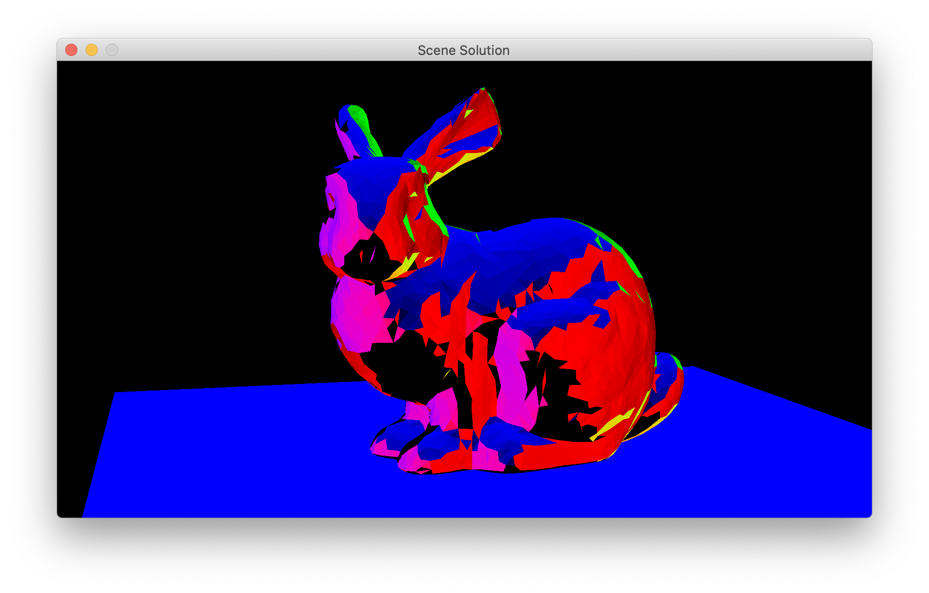
Think through the data that you need for shading (the parameters of the shading model, the surface normal, a flag to distinguish pixels that see the surface from pixels that see the background). Some of the data is 3-component RGB colors or x,y,z vectors; some others are just scalars. Make a plan to pack the information into a few RGBA images; for instance, I used one texture for the diffuse color, one for the specular parameters, one for the surface normal, and stashed the last couple of things in the alpha channels. (I did have some channels left unused.) For performance we usually use 8-bit fixed-point values for these buffers, which means the values need to be manipulated to fit into the range [0,1]. (This is just like storing unit-vector normals in a normal map.)
Note that storing the surface position is not necessary, since it can be recovered from the fragment’s screen space coordinates and depth. Also, it is difficult to store positions in a fixed-point buffer because the coordinates are not naturally limited to a fixed range.
Make a simple fragment shader that takes the same inputs as your
forward rendering shader but writes them (suitably encoded) into several
output colors. When setting up the output variables for the shader, you
will have several of type vec4; the simplest way to map
these to the framebuffer attachments is to use a fixed layout with the
specifier layout(location = n), in the same way as we did
for the vertex shader inputs.
On the C++ side, change your framebuffer so that it allocates the
right number of color attachments. You will need to call glDrawBuffers
to tell OpenGL which of the buffers you want to write to. Then set up
your final pass to read from each of the buffers in turn and display
them so that you can eyeball that you have the right values. Don’t
forget to think about checking the normally invisible values you stored
in the alpha channels. Your images may not be the same as mine, since
your G-buffer layout and/or encoding might be different, but here are
the contents of the three buffers in my solution: 0 1 2.
2.3 Render a point light
Now let’s get the deferred pipeline up to where the forward pipeline was. Add a shading pass in between the geometry pass and the post-processing pass that does the same lighting calculations as in the forward shader, writing the linear (I mean not gamma-corrected) result to its output that will be later read by the sRGB shader. (We want to keep this intermediate image buffer linear because we will do pixel arithmetic to accumulate the results of several lights, and we will get wrong answers if we do this arithmetic on gamma-corrected pixel values.) You will need to allocate a texture for the intermediate image (I’ll call it the accumulation buffer because we will be using it to sum up multiple lights later). It is possible to use the same FBO and attach different textures to it, but the way the Framebuffer class works, it’s simplest to use a second FBO that owns the accumulation texture so that you can use the second constructor and not worry about separately creating the textures. Use a floating-point format here since we will want high dynamic range pixels later.
First ensure your data is flowing properly: set up your shading pass to copy directly from each gbuffer in turn to the output, and ensure you can match the output of the previous step. This will flush out problems with getting the textures bound to the right GLSL samplers or with routing the output of this pass to your post-processing pass.
Next implement simple diffuse shading with a fixed light in direction (1,1,1) (ref), then with the actual light source position and intensity (ref). (At this point you will find you need the eye space position of the fragment; you can compute this by working out the fragment’s position in NDC, then transforming it by the inverse projection matrix. Do not forget you need to divide by w after a perspective transformation. There’s a little more discussion in the last step below.) Finally, add the specular component (ref). Now your deferred pipeline should exactly match the output of your forward pipeline from week 1, up to quantization differences that are barely visible when toggling back and forth between the two modes. (It’s an interesting experiment to try switching the different textures of the G-buffer to floating-point to see where the quantization errors are affecting your result.)
2.4 Sum multiple lights
This step is pretty simple: support multiple lights by adding them in multiple passes. The key parts are:
- In your C++, loop over the lights in the scene, running the shading pass for each one.
- Clear your accumulation buffer beforehand, and set the blending mode
using
glEnableandglBlendFuncso that the successive passes will be added up. Don’t forget to disable blending when you are done, since it will cause wrong results in other passes if left enabled.
Test this step by temporarly changing the type of the area light in the bunny scene to “point”. Here is a reference with both lights, and a different viewpoint.
2.5 Render shadow maps
Next let’s get our point lights to cast shadows by using shadow maps. Since we are rendering one light at a time, we can render each shadow map just before is is used; there is not a need to have all the shadow maps available at the same time. So the overall process looks like:
- Deferred pass: render geometry from camera view, write surface info to G-buffers.
- Clear accumulation buffer.
- For each light:
- Shadow pass: render geometry from light view, producing only a depth buffer.
- Lighting pass: render full screen quad, compute lighting and add to accumulation buffer.
- Color correction pass: convert accumulation buffer values to sRGB, write to default framebuffer.
For this process you need three different sets of buffers (which I attached to three different FBOs): the G-buffer, the shadow map, and the accumulation buffer. Plus of course the default framebuffer where you write the final output.
Now add the shadow pass. This involves:
- Create a framebuffer for this pass that has no color attachments and only a depth attachment.
- Create a shader program for this pass. The vertex shader is totally standard: it just needs to transform the position to NDC. The fragment shader is completely trivial: it takes no inputs, has no uniforms, and doesn’t even have to write a fragment color. It just has to be there.
- Draw the geometry in the same way you do for the first pass. You might need to add a little logic to avoid passing in uniforms that are not going to be used.
Possibly the trickiest part is what to pass in for the viewing and projection matrices. The easiest way to get these is to reuse the camera class, which already knows how to compute viewing and projection matrices, by creating a camera located at the light and looking towards the scene.
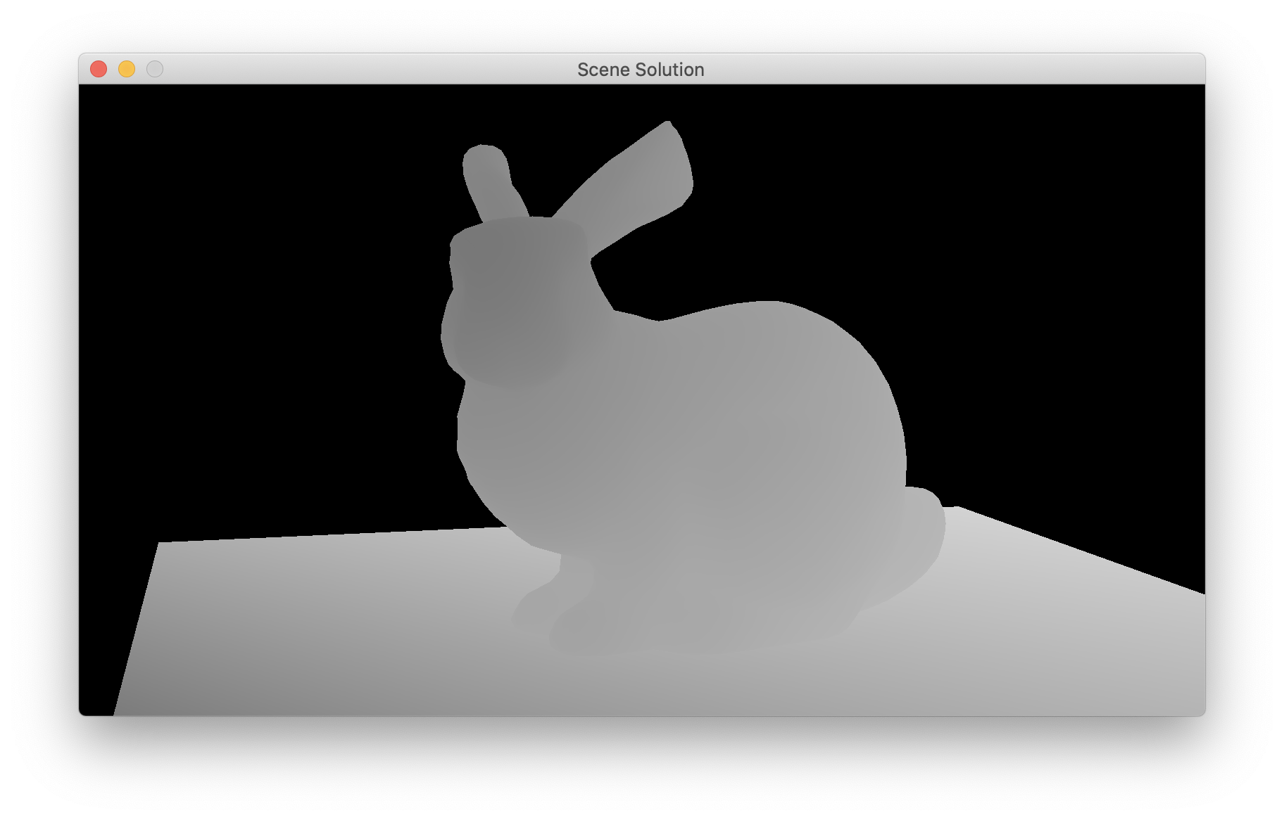
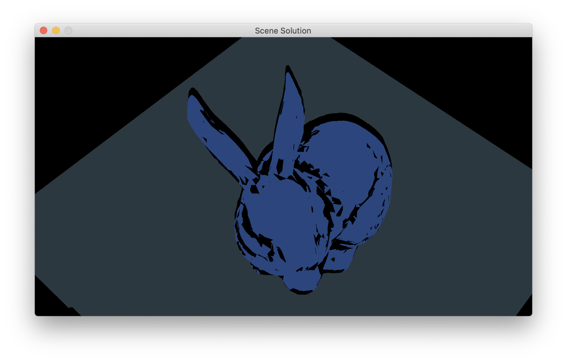
After you add the shadow pass, make sure that the existing lighting pass still works (it should still produce the same output, since it doesn’t actually use the shadow map yet, but it’s easy to disturb the OpenGL state so that you break the lighting pass and it’s nice to fix those problems now). Next, modify your gamma-correction pass to read from the shadow map and display the depth as a greyscale value, so you can get some evidence your shadow pass is working before you try to use the buffer for shadows.
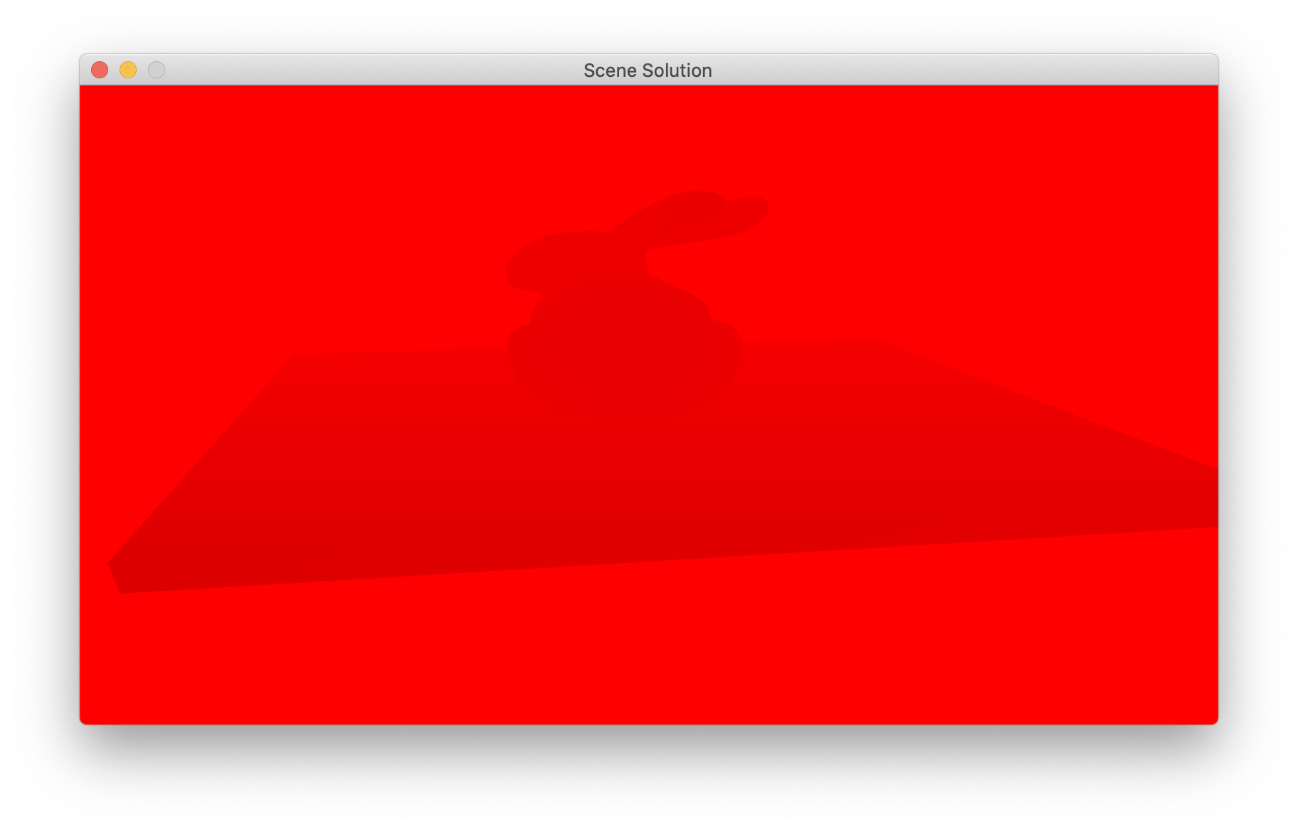
Here is a reference for what my solution produced. It depends on the view parameters for the light source; I pointed the light at the origin, with +y up, used near and far distances of 1 and 20 and used a square, 1 radian field of view. Note that it looks red because when you bind a 1-channel depth texture, the sampler will put the value in the first component of the vector it returns. (A general note about visualizing depth maps: depending on the near and far distances, the depths may be very bunched up near 0 or 1. For instance try looking at the depth map for the scene camera in the bunny scene by reading from the depth texture of your G-buffer; you will see it looks nearly constant, and you might think it is wrong. But if you modify your fragment shader to stretch the values from 0.95 to 1 out to fill the range from 0 to 1, you’ll see it is fine. The cause of this bunching is that the near distance for this camera is set pretty low.)
2.6 Render shadows
Once you have this map looking reasonable it’s time to add shadows to your point light shader. To determine whether a fragment is in shadow, you use a long chain of transforms:
- From the FSQ texture coordinates and the depth stored in the G-buffer, get the NDC coordinates of the fragment by scaling from [0,1] to [-1,1].
- Use the projection and viewing matrices of the scene camera to go from NDC to eye space to world space.
- Use the viewing and projection matrices of the light to go from world space to light space to light NDC.
- Get the shadow texture coordinates and the fragment shadow depth by scaling from [-1,1] to [0,1].
(Do not forget you need to divide by w after a perspective transformation.) Finally, use the x and y shadow coordinates to look up in the shadow map; then compare the z shadow map depth to the fragment shadow depth; you are in shadow if the shadow map depth is significantly less than the fragment’s shadow depth.
This is just a few lines of code, but it does have many places to make errors and is tricky to debug. So here is a recommended testing sequence; all reference images computed with only the point light in the bunny scene enabled.
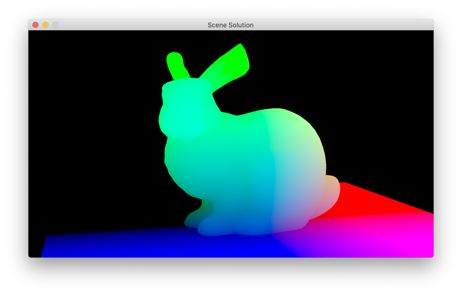
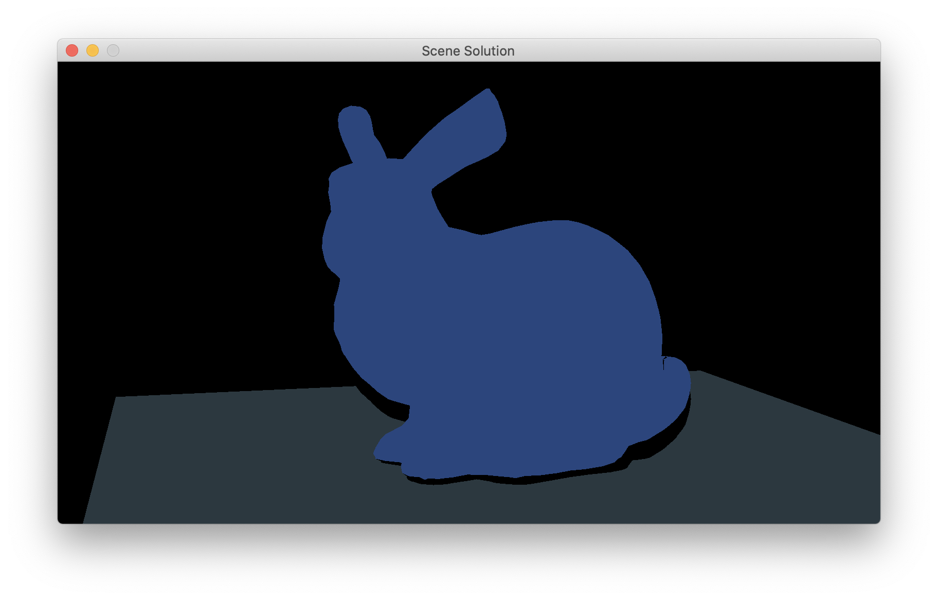
- Compute the world space position of the fragment and write that as your RGB result (ref).
- Compute the light-NDC position of the fragment and write that as your RGB result (ref).
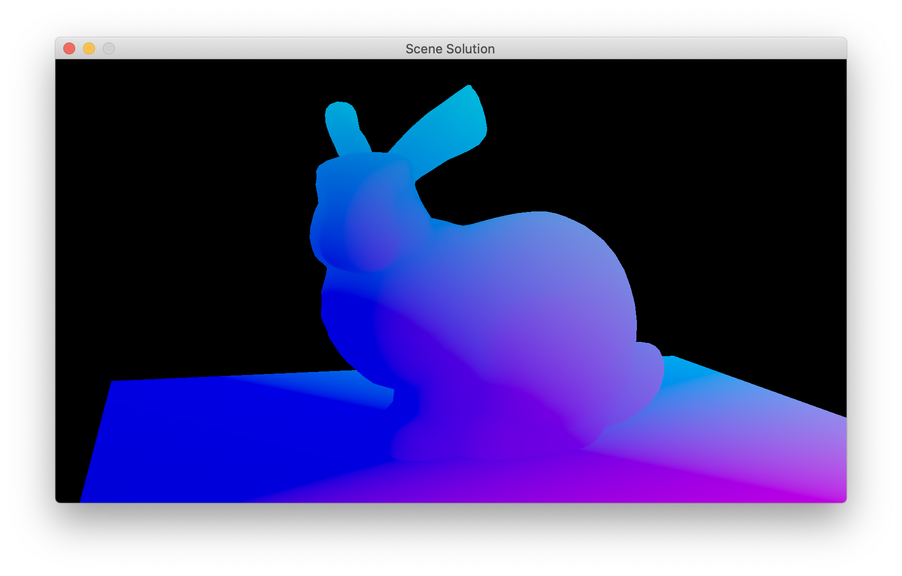
- Compute the light depth (in the range 0 to 1) and write that as a grayscale result (ref; scaled to map [0.8,1] to [0,1]).
- Look up the shadow map depth (in the range 0 to 1) and write that as a grayscale result (ref; scaled to map [0.8,1] to [0,1]).
These last two images should be the same color where the surface is not in shadow. All that remains is to compare these last two values with a bias to decide when you are in shadow.
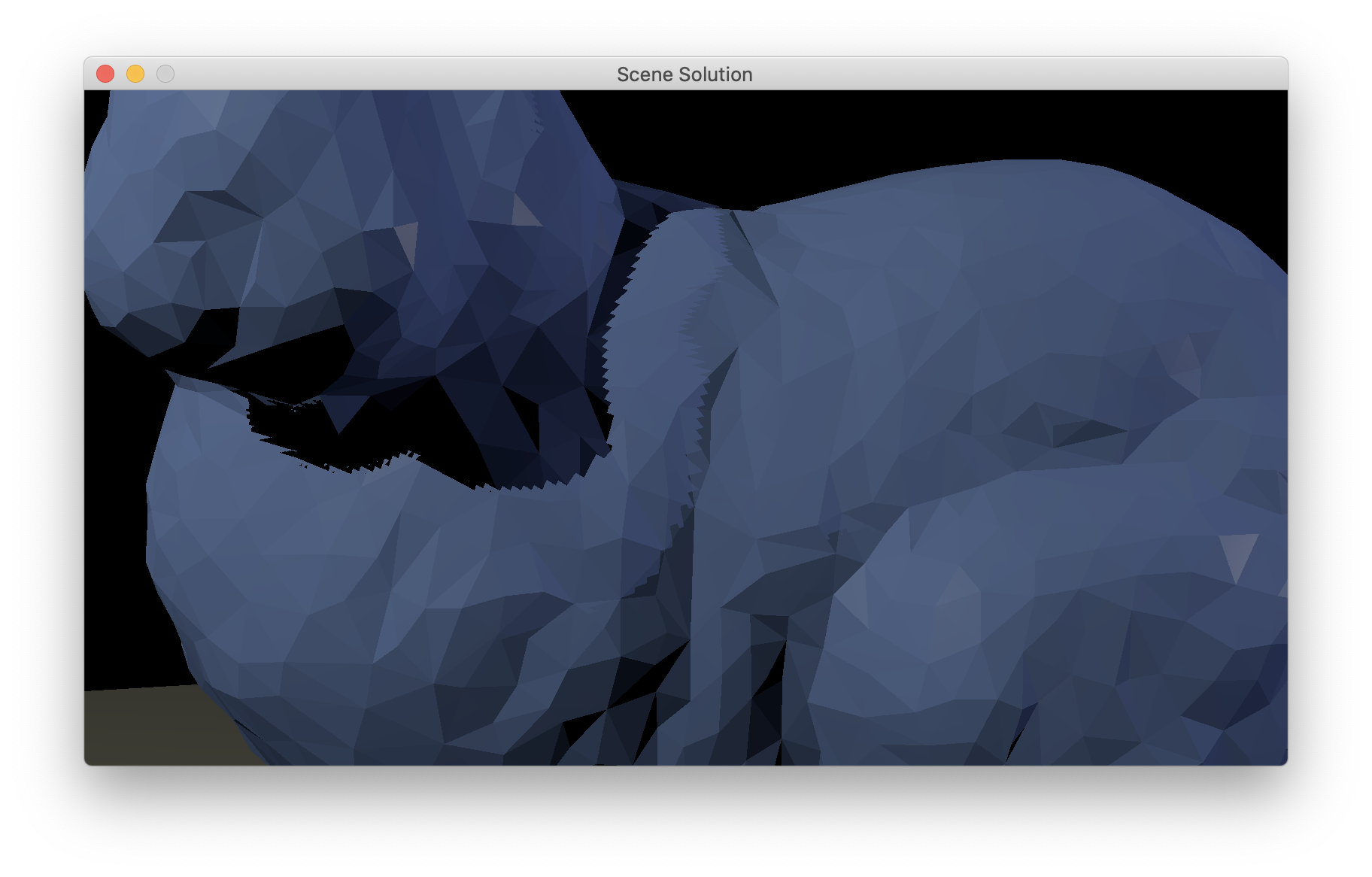
With the two lights in the bunny scene, the shadow map view parameters mentioned above, 1024 by 1024 shadow map resolution, and bias of 0.01, I get an image like this with a pretty jaggy shadow if you zoom in (ref).
Take a few minutes to enjoy your creation! Load up some of the other scenes; make keyboard or Nanogui widget controls for some of the parameters (bias, shadow map resolution, shadow view parameters near/far/fov). Play with them to get a sense for how the technique behaves.
This is the checkpoint for Week 2. You should have this much working on Mar 24 and hand in a very short video showing it off.
2.7 A few pitfalls to avoid
A few random pitfalls I and previous students have encountered, mapped here in case it helps you not fall into them:
- In the various methods (e.g.
Program.uniform) that are overloaded using GLM argument types, you might find the compiler does not know how to match the result of an expression you think is obviously anglm::mat3, for example, against an argument that has that type. The fix is to either construct a matrix of the type you want from the expression, or just assign the expression to a temporary of the appropriate type, so that it is abundantly clear to the compiler which type you mean. - Quantizing the normals in the 8-bit G-buffer will cause them to be non-unit length; this will cause problems with specular shading (which is exquisitely sensitive to exactly normalized vectors) so you will want to normalize the normal after you decode it from the G-buffer.
- Up until now you might have gotten away without worrying about the
viewport. Nanogui set it to match the window size, and so far every
buffer we have drawn to has been the same size. But now that there is a
shadow buffer, which generally will be a different size, you’ll need to
call
glViewportwhen you are setting up to draw to each buffer. (As a general rule, each time you bind an FBO and plan to draw into it you should consider whether you need to clear the buffer, whether you need to set the viewport, and whether you need to enable or disable some features like the depth test or blending.) - When you are writing diagnostic info into the output from your lighting pass, don’t forget it is adding up contributions from multiple lights (unless you temporarily disable all but one, which is probably a good idea).
3 Ambient illumination and bloom
This week is getting to methods that look more and more like image processing, that take many samples from a neighborhood in a source texture and average them in some way to get a filtered output. The first method is screen-space ambient occlusion, which samples from a pixel’s neighborhood in the depth buffer to decide how much ambient illumination to add. The second is bloom, which samples from a pixel’s neighborhood in the rendered image to decide how much bloom to add.
3.1 Ambient occlusion
3.1.1 Set up an ambient pass.
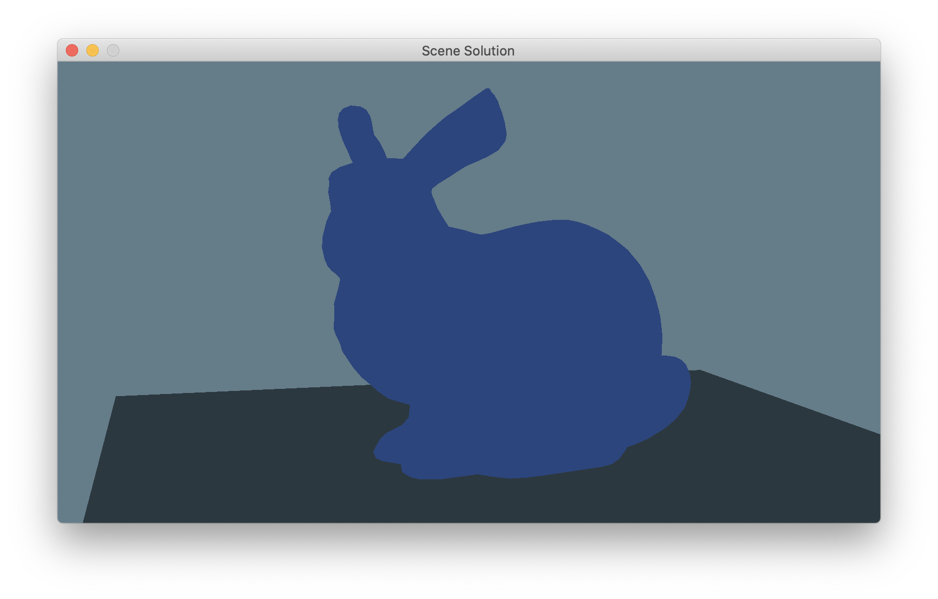
The ambient pass fits into the overall shading pipeline in the same
way as the lighting pass does; in fact, since the ambient light is a
light source in our system, it’s really just a lighting pass for a
different kind of light, which does the same thing but calls a different
shader program and doesn’t do anything with shadow maps. Set up this
pass with a shader that outputs an unoccluded ambient shading component
that is just the product of the ambient radiance, the diffuse
reflectance, and (since the ambient radiance
gets integrated, cosine weighted, over the hemisphere). You should get a
result that adds a
constant-color component to your shading, which looks just like what
your ray tracer will output with the ambient range set to zero. (My
reference image has the other two lights disabled.) It also looks a lot
like a direct readout of the diffuse color G-buffer.
All that remains is to compute an occlusion factor for this ambient light.
3.1.2 Build a surface frame in eye space.
To generate sample points for AO, we need a surface frame much like the one we built in the ray tracer for the same purpose. If we had tangent vectors in our system we’d be just about done already, but since we don’t, we need to build an arbitrarily oriented frame around the surface normal. This is easy to do by starting with the normal and a vector not parallel to it, and doing a few cross products. The recommended way to choose a non-parallel vector is to compare the three components of the normal to find out which is smallest, and use the coordinate axis vector pointing in that direction.
Test this by writing out the pixel’s eye space position and the three vectors of your surface frame, and maybe writing out the dot products between your vectors. Your results for the position and normal should match mine (though the background does not matter) but the results for the tangents can look different and still be correct. (ref: eyepos normal tangent1 tangent2) If one vector is the normal, the pairwise dot products are all zero, and the vectors are unit length, you are good to go.
3.1.3 Test points for occlusion.
SSAO hinges on being able to take a point in the surface frame and
determine whether it is behind the depth buffer or in front. Implement
this test: take a point in the surface
tangent frame, transform it to eye space and then screen space, and look
up in the depth buffer. Compare the buffer depth with the point’s depth,
using a small constant bias (0.00001 should suffice with a 24-bit depth
buffer) to break ties in favor of non-occlusion, so that flat surfaces
don’t get erroneous occlusion on them.
You can compare against my implementation by checking the points
(0.1, 0, 0) (ref), (0,
0.1, 0) (ref), and (0,
0, 0.1) (ref) in the
local frame (I have my in the order:
tangent1, tangent2, normal) for occlusion and computing an all-or
nothing occlusion factor to multiply against the ambient lighting. If
you built your frame the same way I did these could all match; otherwise
the third one (
direction) should match (since the
normal direction is well defined) but the other two will exhibit similar
behavior but different details.
3.1.4 Finish SSAO.
Now you have all the components to put together the SSAO algorithm.
You need a loop that generates random points in the hemisphere, tests
them for occlusion, and uses the fraction of unoccluded points as the
ambient occlusion factor. There are a number of distributions that can
be used to generate these points, but here is a simple one: we are
trying to approximate the occlusion due to cosine-distributed rays like
the ones we used in the ray tracer. So to generate points in the
hemisphere, just generate directions as in the ray tracer (unit vectors
on the hemisphere around the surface normal, distributed proportional to
. You can just
port the code we used for that assignment to GLSL, or use the simpler
math from class. Then generate distances
. Once you have points in
the interior of the unit hemisphere, you can scale them by the occlusion
range so that you are probing at the right scale.
One other tool you’ll need is a pseudorandom number generator. The classic way to do this is to use a GLSL hack whose origins are lost to the mists of time, but which is very widely used for this purpose:
float random(vec2 co) {
    return fract(sin(dot(co.xy,vec2(12.9898,78.233))) * 43758.5453);
}
This hash function takes a 2D position and returns a result that varies very rapidly with that position, so that as long as you call it for different 2D positions it will produce results that are usable as random numbers. It’s not a bulletproof random number generator (don’t use it for cryptographic purposes!) but it suffices for random sampling tasks like this one. You just need to make up a vec2 which will have a different value for every sample for every fragment, by combining the sample counter with your texture coordinate somehow.
This will give you basic SSAO but with some extra haloes at object boundaries (ref). These can be improved by computing the distance between the point you sampled from the depth buffer and the pixel’s position, and not counting the occlusion if this distance is larger than a multiple (I used 4 in the reference) of the occlusion range (ref).
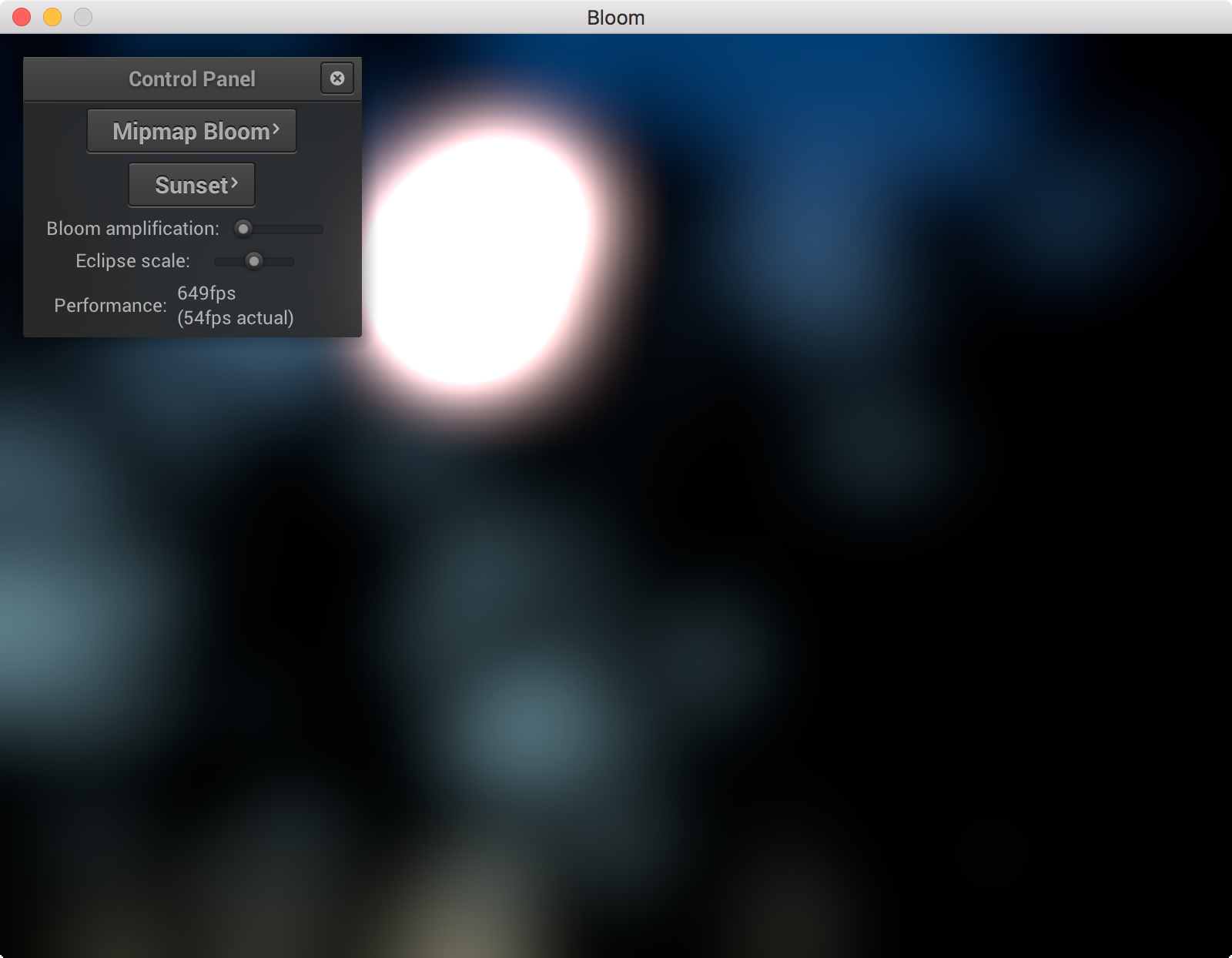
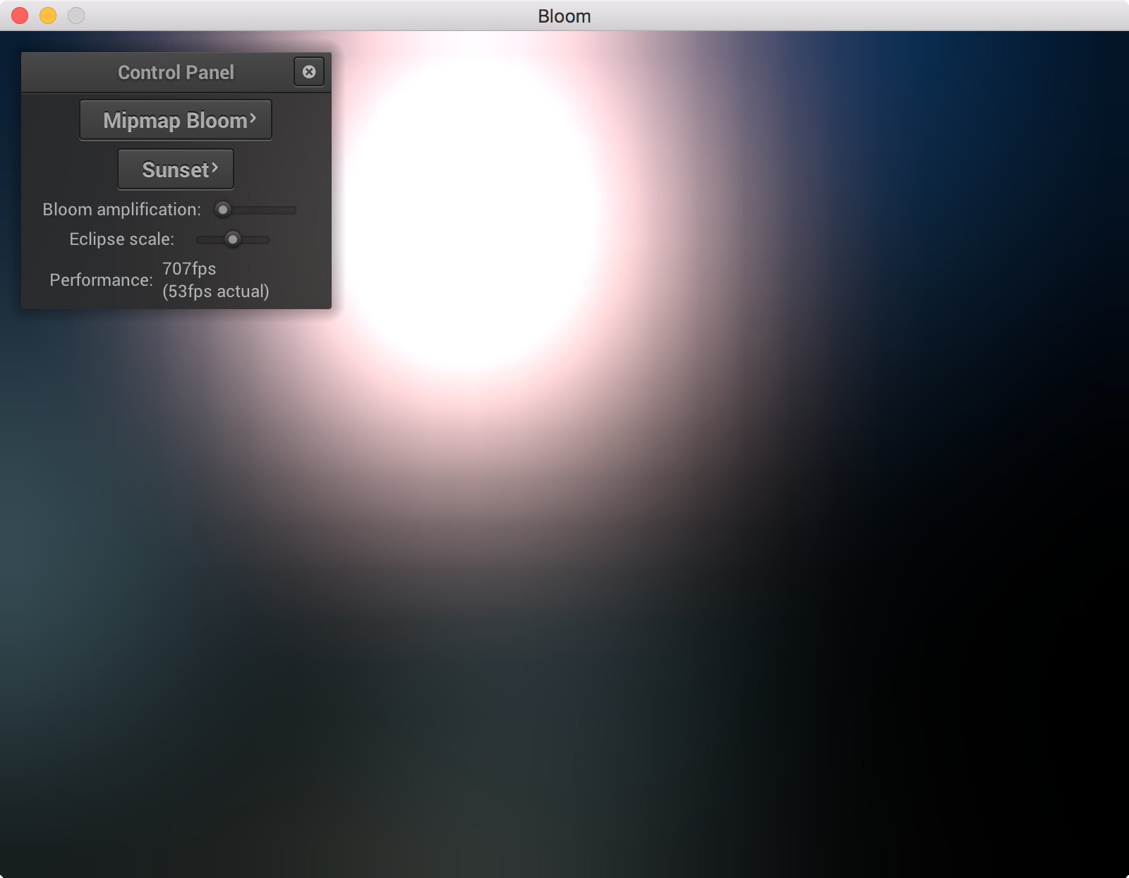
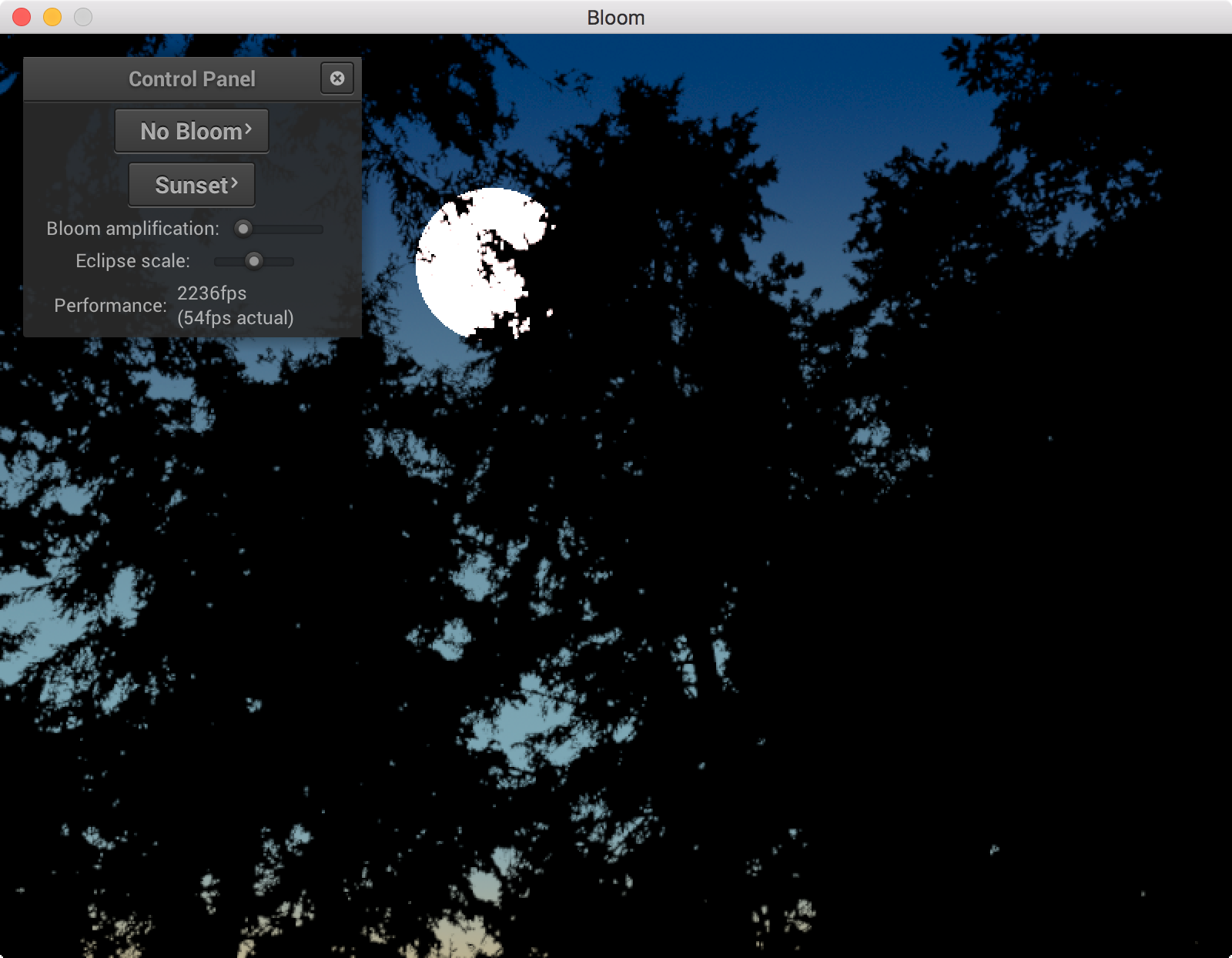
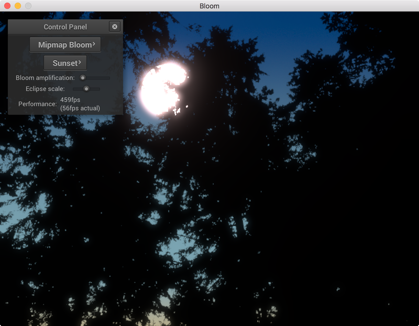
3.2 Bloom filter
Bloom is a visual effect that aims to simulate the phenomenon in which imperfections in the optics of the eye produce halos of light around bright objects. A nice model for this effect is described by Spencer et al.; essentially it causes the image you see to be convolved with a filter that is very sharp at the center but has long, very faint tails.
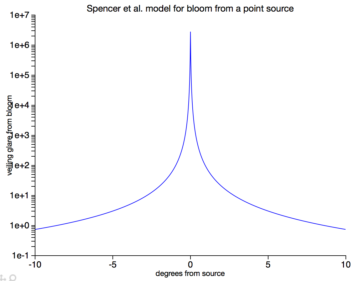
When filtering most parts of the image, it will have essentially no effect, since the tails of the filter are so faint, but when something like the sun comes into the frame, the pixel values are so high that the faint tails of the filter contribute significantly to other parts of the image.
The problem is, this filter is too big to work with directly: the tails should extend a large fraction of the size of the image. And worse, it is not separable. So doing a straight-up space-domain convolution is hopeless.
Instead, we approximate this filter with the sum of an impulse and several Gaussian filters. The result is that the filter we will use is
where is a
normalized Gaussian with standard deviation
.
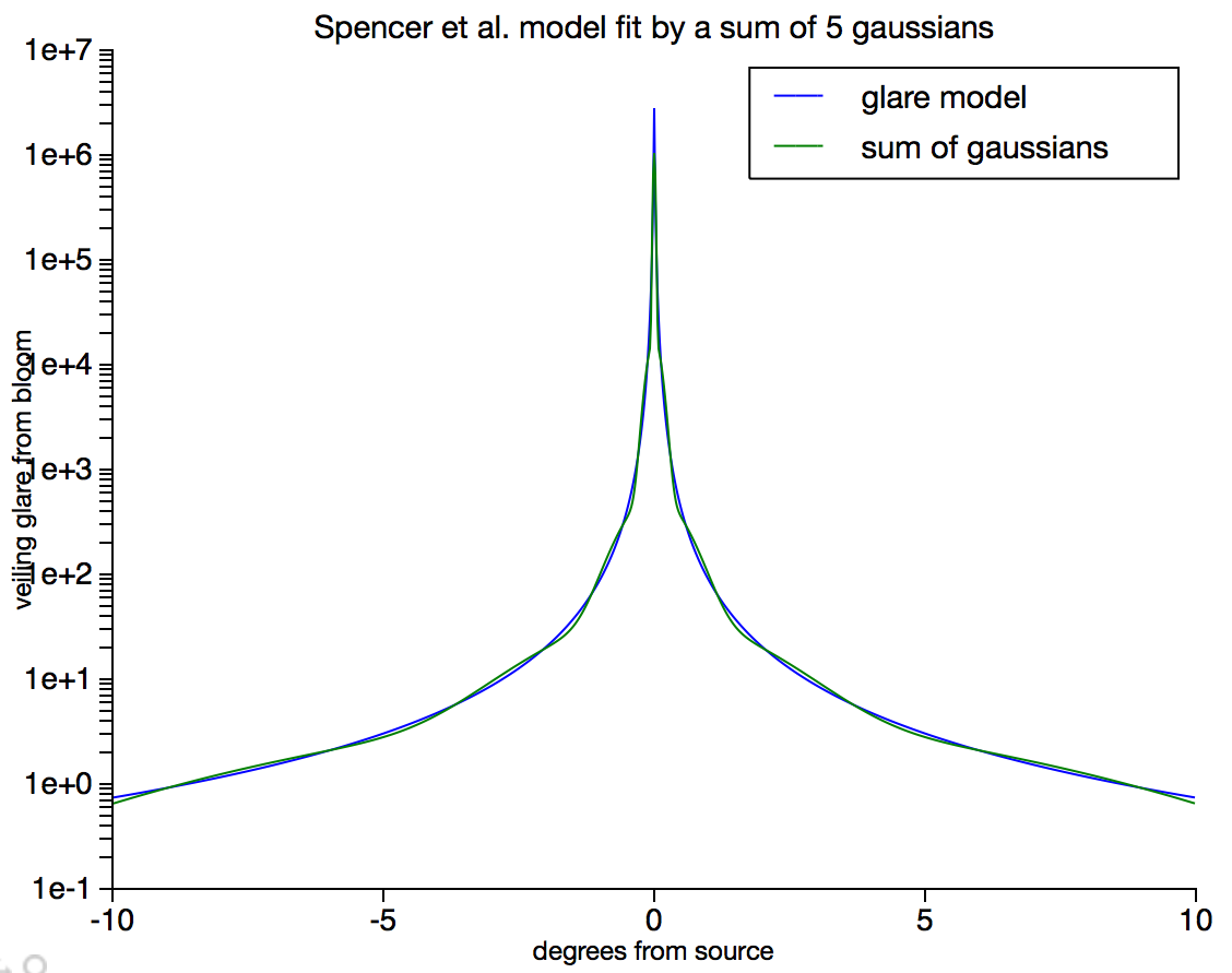
With this approximation in hand, we can convolve the rendered images with 4 Gaussian kernels, each with different width, which is fast since they are separable filters. The results of the convolutions are as follows:
Then to compute the final image we just scale each of these blurred images the coefficients in the equation above, as well as the original image, and add them all up to produce the final image.
In this part we’ll put together an implementation of this model.
3.2.1 Add a sun-sky model.
The first thing we need in order for a bloom filter to be useful is a
bright light source. To this end I added to the RTUtil library a simple
sun-and-sky model based on the Preetham et al. paper
we saw in lecture, which comes in two parts. One is in a fragment shader
function in sunsky.fs; you can call the function
sunskyRadiance(worldDir) to get the sky radiance in a
particular direction. The other is a C++ class RTUtil::Sky
which is able to compute the uniform values needed by the fragment
shader code. See Sky.hpp for brief documentation.
Install the sky model in your program by creating a Sky instance,
linking sunsky.fs into the shader program for some
appropriate pass (I used my ambient pass for this, but the sky could be
its own pass too), and calling sunskyRadiance to get values
for background pixels. To do this you will need to have the world space
direction of the viewing ray for the pixel you are rendering. But you
have the fragment position in screen space, and if you make the inverse
projection and inverse view matrices available, you can use a similar
approach as in the lighting passes to transform points from screen space
to world space. You can’t directly transform a ray direction through a
perspective matrix, but a feasible approach to do this is to ttransform
points on the near and far plane at your fragment position, and subtract
them in world space to get the direction.
With this done you should find there is a sky in the background of your scene (ref). It is fun to adjust the sun angle to see the sunrise/sunset. You probably will want an exposure adjustment for this part, since you now have HDR images. Note that the sky has an arbitrary scale factor that is set to bring the sky into the [0, 1] range that we have been using for ambient lighting, but you can adjust it as needed. Also the sun radiance is completely arbitrary, but set to a number big enough to get dramatic bloom effects but small enough not to overflow half-precision floating point.
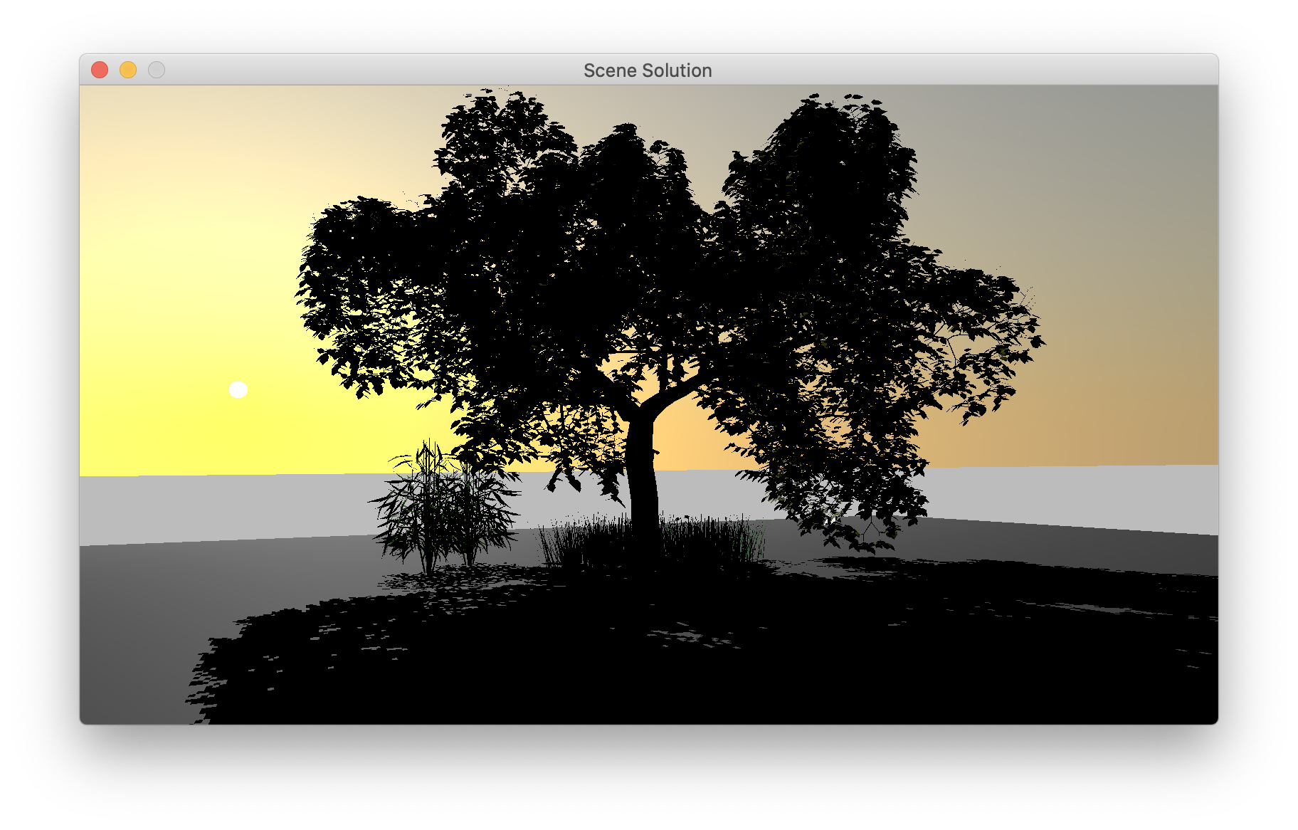
3.2.2 Implement a blur pass
The core operation in our bloom filter is a gaussian blur, which for performance should be done separably in two passes (see slides 21-22 in this lecture if you forget how this works). I’m providing a shader in blur.fs to do this fairly standard 1D blurring operation. Its parameters include the standard deviation of the filter, a floating point number measured in pixels; the radius of the box over which the filter will be evaluated, an integer also measured in pixels; the mipmap level it should read from in the input (zero to just read from the full resolution texture); and a 2D vector that gives the direction along which the blur should happen (normally (1,0) or (0,1)).
To get started, implement a blurring pass that will simply take the result of rendering and apply a Gaussian blur to it. To do this you will need at least one additional color texture to hold the intermediate result (remember you are not allowed to write to the same texture you are reading from). Do a full-screen-quad pass that blurs vertically, reading from the rendered image and writing to your intermediate buffer, then a second pass that blurs horizontally, reading from the intermediate buffer and writing back to the rendered image. If you enable this pass you should see the image getting blurry (how blurry depends on how you choose sigma). This blurring will make it obvious that the sun is many times brighter than just white. Play with the sigma and radius parameters; you’ll see that Gaussian blurs are nice and round, but only as long as the radius is large enough (otherwise the Gaussian filter gets trimmed to a square and the result starts to look square-ish). A good conservative rule is to keep the radius larger than three times the standard deviation.
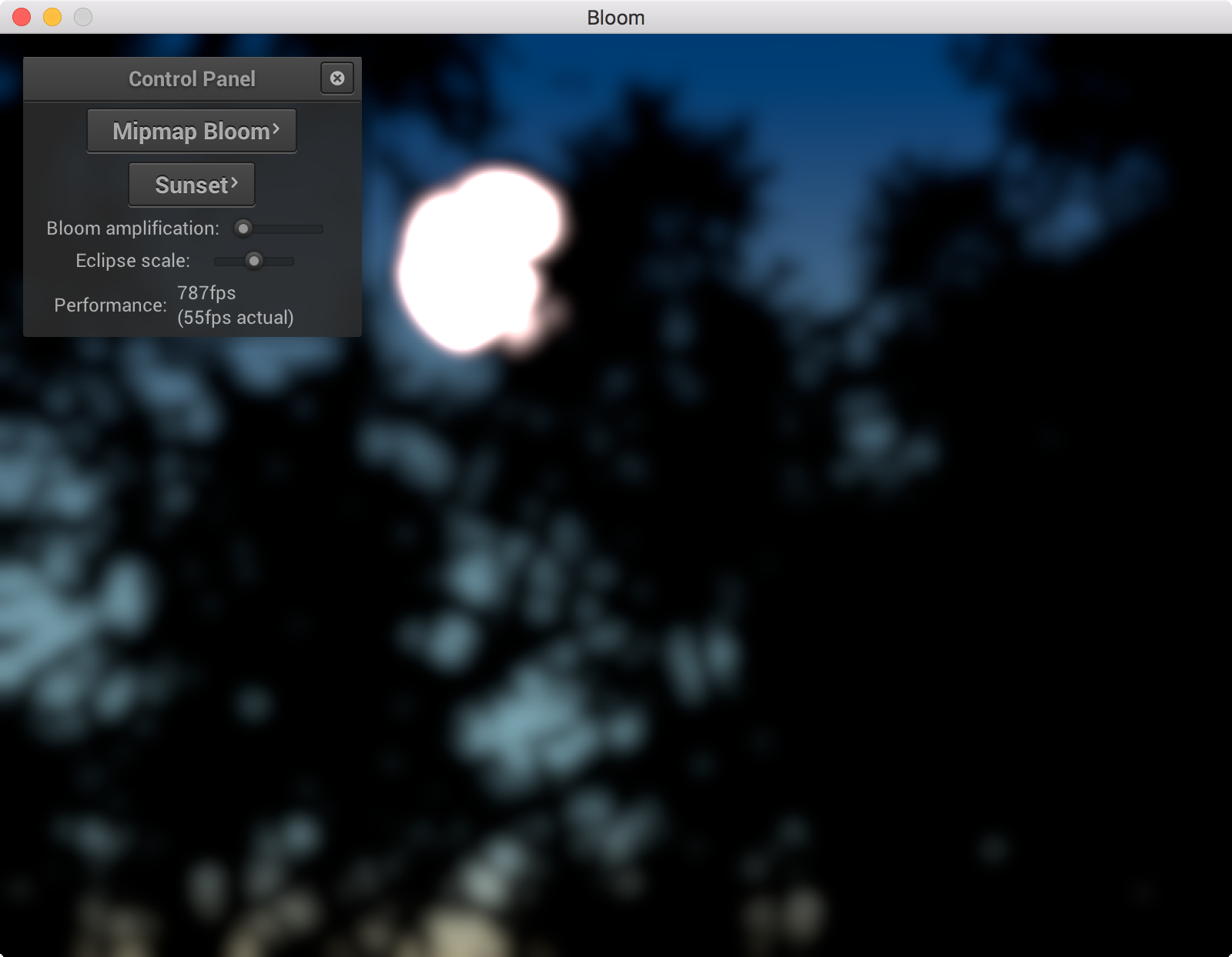
3.2.3 Apply blur to mipmap levels
You’ll notice that with your single-resolution blur pass, performance
really suffers if you make the radius very big. This is because the blur
filter, even though it’s separable, has to read 2*radius+1 pixels from
the source image for every pixel in the output, and with
limited texture bandwidth (and ineffective caches with each fragment
touching so much memory) this gets very slow. The solution is to do
large blurs at a lower resolution. To blur the image with a gaussian of
stdev : downsample the image
by a factor of
, blur with stdev
, then
upsample by a factor of
to get back to the original
resolution.
The nice thing is that OpenGL already contains the machinery for
downsampling and upsampling efficiently, in the implementation of
mipmaps. If you simply call generateMipmaps on your
texture, OpenGL will build an image pyramid for you, so that at level
of the mipmap you have an image
downsampled by a factor of
, and you can read or write
these lower resolution images directly. Normally when you read textures
using texture, OpenGL will automatically decide what mipmap level to
use, but you can also read from the mipmap as a set of separate textures
using the textureLod GLSL function, and texture interpolation handles
upsampling as needed. When you write to a texture by binding it as a
framebuffer attachment, you normally bind the full resolution texture
(aka. level 0 of the mipmap), but you can also specify a different
mipmap level when you bind a texture using
glFramebufferTexture2D (in our framwork you just supply the
mipmap level as the argument to Framebuffer::bind).
Two gotchas with reading mipmap levels directly. (1) For
textureLod to work you need to have a mipmapping
minification mode set (e.g. LINEAR_MIPMAP_LINEAR). This
seems like it might not matter since you are not using mipmap
interpolation, but if you have a single-resolution mode set
(e.g. LINEAR) then it just doesn’t turn on the mipmap machinery at all.
(2) If you try to bind a texture for which you have never generated
mipmaps to a framebuffer, you will end up with an OpenGL error (Invalid
Framebuffer Operation), because the mipmap levels physically do not
exist yet.
There are various ways to set up the blur filter; the strategy I used is:
- Allocate two intermediate textures the same size as the input texture, and run generateMipmap on all three textures.
- Blur pass: for each
choose an appropriate
, and blur mipmap level
- Merge pass: Read from all four blurred mipmap levels and compute a weighted combination with the original image, back in the input texture.
To get started with this, set up the merge pass so it just writes one
level at a time straight to the output. Then you can verify you see
blurred content in the levels where you wrote it, and nothing in the
other levels. I did this first with the texture filtering modes all set
to GL_NEAREST_MIPMAP_NEAREST which makes it obvious what
level you are reading from (since you see squares of size ). But don’t forget to put
it back to
GL_LINEAR_MIPMAP_LINEAR because the final
results will be much smoother.
3.2.4 Finish the bloom filter
Once you can see the individual blurred images, write the real merge shader that computes the correct weighted combination. There are a few ways to do this; what I did was to render a linear combination of the four relevant levels of the blur buffer into the input texture, setting up blending and alpha values to give the correct weight to the blurred and original contributions.
4 Handing in
Handing in is much the same as for the ray tracing assignment:
Before the deadline, submit your C++ code by providing a link to the particular commit of your github repo that you want to hand in.
Before the deadline, submit some output images for our test scenes.
One day after the deadline, submit a 2- to 5-page PDF report and a 2- to-5-minute video demo that cover the following topics:
- The design and implementation of your program.
- Demonstrations of your interactive rendering in action.
- What works and doesn’t, if not everything works perfectly. This could include illustrations showing that you successfully achieved some of the intermediate steps in our guidelines.
Think of these three channels as your way to provide us evidence that your program is designed nicely and works as intended.