Lecture 9: SVM

The Support Vector Machine (SVM) is a linear classifier that can be viewed as an extension of the Perceptron developed by Rosenblatt in 1958. The Perceptron guaranteed that you find a hyperplane if it exists. The SVM finds the maximum margin separating hyperplane.

We define a linear classifier: $h(\mathbf{x})=sign(\mathbf{w}^{T}\mathbf{x}+b)$ and we assume that our labels are within $\{+1,-1\}$.

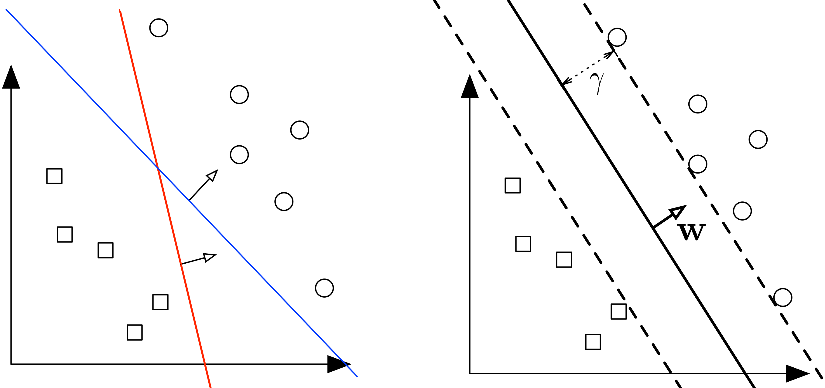
Figure 1: (Left:) Two different separating hyperplanes for the same data set. (Right:) The maximum margin hyperplane. The margin, $\gamma$, is the distance from the hyperplane (solid line) to the closest points in either class (which touch the parallel dotted lines).

Typically, if a data set is linearly separable, there are infinitely many separating hyperplanes. A natural question to ask is:

Question: What is the best separating hyperplane?

SVM Answer: The one that maximizes the distance to the closest data points from both classes. We say it is the hyperplane with maximum margin.

Margin

We already saw the definition of a margin in the context of the Perceptron. A hyperplane is defined through $\mathbf{w},b$ as a set of points such that $\mathcal{H}=\left\{\mathbf{x}\vert{}\mathbf{w}^T\mathbf{x}+b=0\right\}$. Let the margin $\gamma$ be defined as the distance from the hyperplane to the closest point across both classes.

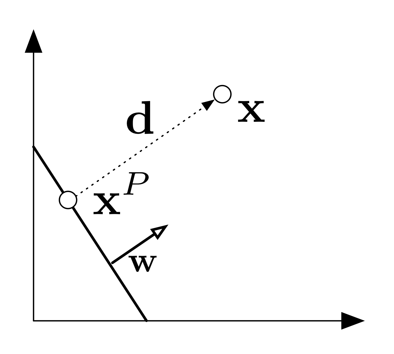
What is the distance of a point $\mathbf{x}$ to the hyperplane $\mathcal{H}$?
Consider some point $\mathbf{x}$. Let $\mathbf{d}$ be the vector from $\mathcal{H}$ to $\mathbf{x}$ of minimum length. Let $\mathbf{x}^P$ be the projection of $\mathbf{x}$ onto $\mathcal{H}$. It follows then that:
$\mathbf{x}^P=\mathbf{x}-\mathbf{d}$.
$\mathbf{d}$ is parallel to $\mathbf{w}$, so $\mathbf{d}=\alpha\mathbf{w}$ for some $\alpha\in\mathbb{R}$.
$\mathbf{x}^P\in\mathcal{H}$ which implies $\mathbf{w}^T\mathbf{x}^P+b=0$
therefore $\mathbf{w}^T\mathbf{x}^P+b=\mathbf{w}^T(\mathbf{x}-\mathbf{d})+b=\mathbf{w}^T(\mathbf{x}-\alpha\mathbf{w})+b=0$
which implies $\alpha=\frac{\mathbf{w}^T\mathbf{x}+b}{\mathbf{w}^T\mathbf{w}}$
The length of $\mathbf{d}$:
$\left \| \mathbf{d} \right \|_2=\sqrt{\mathbf{d}^T\mathbf{d}}=\sqrt{\alpha^2\mathbf{w}^T\mathbf{w}}=\frac{\left | \mathbf{w}^T\mathbf{x}+b \right |}{\sqrt{\mathbf{w}^T\mathbf{w}}}=\frac{\left | \mathbf{w}^T\mathbf{x}+b \right |}{\left \| \mathbf{w} \right \|_{2}}$
Margin of $\mathcal{H}$ with respect to $D$: $\gamma(\mathbf{w},b)=\min_{\mathbf{x}\in D}\frac{\left | \mathbf{w}^T\mathbf{x}+b \right |}{\left \| \mathbf{w} \right \|_{2}}$

By definition, the margin and hyperplane are scale invariant: $\gamma(\beta\mathbf{w},\beta b)=\gamma(\mathbf{w},b), \forall \beta \neq 0$

Note that if the hyperplane is such that $\gamma$ is maximized, it must lie right in the middle of the two classes. In other words, $\gamma$ must be the distance to the closest point within both classes. (If not, you could move the hyperplane towards data points of the class that is further away and increase $\gamma$, which contradicts that $\gamma$ is maximized.)

Max Margin Classifier

We can formulate our search for the maximum margin separating hyperplane as a constrained optimization problem. The objective is to maximize the margin under the constraints that all data points must lie on the correct side of the hyperplane: $$ \underbrace{\max_{\mathbf{w},b}\gamma(\mathbf{w},b)}_{maximize \ margin} \textrm{such that} \ \ \underbrace{\forall i \ y_{i}(\mathbf{w}^Tx_{i}+b)\geq 0}_{separating \ hyperplane} $$ If we plug in the definition of $\gamma$ we obtain: $$ \underbrace{\max_{\mathbf{w},b}\underbrace{\frac{1}{\left \| \mathbf{w} \right \|}_{2}\min_{\mathbf{x}_{i}\in D}\left | \mathbf{w}^T\mathbf{x}_{i}+b \right |}_{\gamma(\mathbf{w},b)} \ }_{maximize \ margin} \ \ s.t. \ \ \underbrace{\forall i \ y_{i}(\mathbf{w}^Tx_{i}+b)\geq 0}_{separating \ hyperplane} $$ Because the hyperplane is scale invariant, we can fix the scale of $\mathbf{w},b$ anyway we want. Let's be clever about it, and choose it such that $$\min_{\mathbf{x}\in D}\left | \mathbf{w}^T\mathbf{x}+b \right |=1.$$ We can add this re-scaling as an equality constraint. Then our objective becomes: $$\max_{\mathbf{w},b}\frac{1}{\left \| \mathbf{w} \right \|_{2}}\cdot 1 = \min_{\mathbf{w},b}\left \| \mathbf{w} \right \|_{2} = \min_{\mathbf{w},b} \mathbf{w}^\top \mathbf{w}$$ (Where we made use of the fact $f(z)=z^2$ is a monotonically increasing function for $z\geq 0$ and $\|\mathbf{w}\|\geq 0$; i.e. the $\mathbf{w}$ that maximizes $\|\mathbf{w}\|_2$ also maximizes $\mathbf{w}^\top \mathbf{w}$.)

The new optimization problem becomes:
$$ \begin{align} &\min_{\mathbf{w},b} \mathbf{w}^\top\mathbf{w} & \\ &\textrm{s.t. } \begin{matrix} \forall i, \ y_{i}(\mathbf{w}^T \mathbf{x}_{i}+b)&\geq 0\\ \min_{i}\left | \mathbf{w}^T \mathbf{x}_{i}+b \right | &= 1 \end{matrix} \end{align}$$

These constraints are still hard to deal with, however luckily we can show that (for the optimal solution) they are equivalent to a much simpler formulation. (Makes sure you know how to prove that the two sets of constraints are equivalent.) $$ \begin{align} &\min_{\mathbf{w},b}\mathbf{w}^T\mathbf{w}&\\ &\textrm{s.t.} \ \ \ \forall i \ y_{i}(\mathbf{w}^T \mathbf{x}_{i}+b) \geq 1 & \end{align} $$

This new formulation is a quadratic optimization problem. The objective is quadratic and the constraints are all linear. We can be solve it efficiently with any QCQP (Quadratically Constrained Quadratic Program) solver. It has a unique solution whenever a separating hyper plane exists. It also has a nice interpretation: Find the simplest hyperplane (where simpler means smaller $\mathbf{w}^\top\mathbf{w}$) such that all inputs lie at least 1 unit away from the hyperplane on the correct side.

SVM with soft constraints

If the data is low dimensional it is often the case that there is no separating hyperplane between the two classes. In this case, there is no solution to the optimization problems stated above. We can fix this by allowing the constraints to be violated ever so slight with the introduction of slack variables: $$\begin{matrix} \min_{\mathbf{w},b}\mathbf{w}^T\mathbf{w}+C\sum_{i=1}^{n}\xi _{i} \\ s.t. \ \forall i \ y_{i}(\mathbf{w}^T\mathbf{x}_{i}+b)\geq 1-\xi_i \\ \forall i \ \xi_i \geq 0 \end{matrix}$$ The slack variable $\xi_i$ allows the input $\mathbf{x}_i$ to be closer to the hyperplane (or even be on the wrong side), but there is a penalty in the objective function for such "slack". If C is very large, the SVM becomes very strict and tries to get all points to be on the right side of the hyperplane. If C is very small, the SVM becomes very loose and may "sacrifice" some points to obtain a simpler (i.e. lower $\|\mathbf{w}\|_2^2$) solution.

Unconstrained Formulation:

Let us consider the value of $\xi_i$ for the case of $C\neq 0$. Because the objective will always try to minimize $\xi_i$ as much as possible, the equation must hold as an equality and we have: $$ \xi_i=\left\{ \begin{array}{cc} \ 1-y_{i}(\mathbf{w}^T \mathbf{x}_{i}+b) & \textrm{ if $y_{i}(\mathbf{w}^T \mathbf{x}_{i}+b)<1$}\\ 0 & \textrm{ if $y_{i}(\mathbf{w}^T \mathbf{x}_{i}+b)\geq 1$} \end{array} \right. $$ This is equivalent to the following closed form: $$ \xi_i=\max(1-y_{i}(\mathbf{w}^T \mathbf{x}_{i}+b) ,0). $$ If we plug this closed form into the objective of our SVM optimization problem, we obtain the following unconstrained version as loss function and regularizer: $$ \min_{\mathbf{w},b}\underbrace{\mathbf{w}^T\mathbf{w}}_{l_{2}-regularizer}+ C\ \sum_{i=1}^{n}\underbrace{\max\left [ 1-y_{i}(\mathbf{w}^T \mathbf{x}+b),0 \right ]}_{hinge-loss} \label{eq:svmunconst} $$ This formulation allows us to optimize the SVM paramters ($\mathbf{w},b$) just like logistic regression (e.g. through gradient descent). The only difference is that we have the hinge-loss instead of the logistic loss.

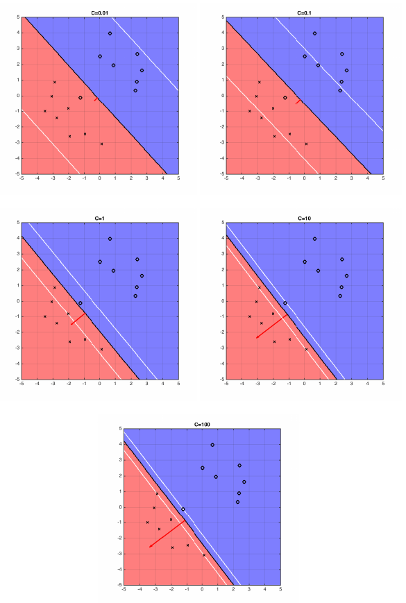
Figure 2: The five plots above show different boundary of hyperplane and the optimal hyperplane separating example data, when C=0.01, 0.1, 1, 10, 100.