
Example 1: A root finding environment.
In this example, we will implement a simple interactive graphic
application in MATLAB. This will illustrate many of the graphics
concepts we have introduced in this part while at the same time
demonstrate the simplest of MATLAB's GUI capabilities, function
ginput.
The problem we want to solve is the following:
Usually, in
applications of mathematics to engineering one wants to find all roots
of a continuous function on a given interval. Recall that a root of a
function f on the interval [a,b] is a
number x in this interval such that f(x) ==
0. MATLAB of course has built-in procedures for finding a root
of a function on a given interval. Alternatively, one can implement a
simple procedure such as the Bisection method that
always finds a root of a continuous function f on an
interval [L,R] provided that f(L) and
f(R) have opposite signs. However, the root returned by
such procedures can be any of the many possible roots in the interval
and the user has little control over which of them is returned. Also,
it is a priori impossible to have the procedure return all roots
contained in the interval.
One way around this problem is to let the user specify a series of narrower intervals containing only one root each and invoke the root finding procedure on each of them individually. Such intervals are termed bracketing intervals. The problem with this approach is that it places the burden back on the user, as she has to come up with such bracketing intervals and to call the root finding procedure on each of them.
In what follows, we will develop an environment to streamline the procedure of finding all bracketing intervals and the roots on each of them, thus greatly alleviating the burden on the user side.
The basic idea is to let the user locate bracketing intervals by
visual exploration in a zoom-in/zoom-out process driven by mouseclicks
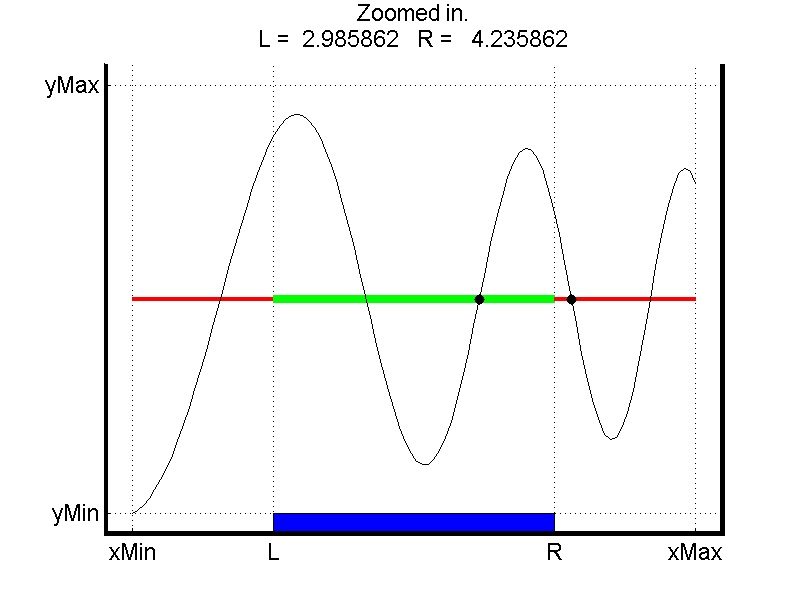
on a carefully designed "bisection window". This bisection window,
shown in the figure below, displays at any point in time a plot of the
function in some interval [xMin, xMax] along with the
roots found so far (marked with black dots in the figure). It also displays
a candidate bracketing interval [L,R] for a root.
This window is interactive in that the user can click on any of a number of different zones and this causes the application to perform one of the possible actions:
- Try to find a root on the interval
[L,R]using the Bisection method. This is triggered by clicking on the blue zone. Recall that for the bisection method to be applicablef(L)andf(R)should have opposite signs. - Zoom-out to a wider interval, triggered by clicking to the left
of
Lor the right ofR. - Zoom-in to a narrower interval, triggered by clicking on a point with
x-coordinate between
LandR. - Quit the application, triggered by clicking on a point with
xcoordinate outside of[xMin, xMax].
To try out the application yourself download the following files
to a directory on your computer and run the command
FindRoots(@MyF, 0,10) FindRoots.m
BWindow.m Bisection.m MyF.m DrawRect.m
A description of each of these files follows:
Function FindRoots
This is driver, i.e. main, function. It takes as a input a
reference to a function whose roots are to be found along with an the
limits for an initial interval [xMin, xMax]. The root
finding procedure will be constrained to this interval.
A reference to a function is constructed by prepending @ to the name of any
built-in or user-defined function. We have provided an example function
MyF but this could be replaced by any continuous function.
FindRoots runs a loop,
executing actions according to the user clicks as described above. At
each iteration it calls function BWindow to refresh the
bisection window and to get a new click from the user. When exiting,
it returns all roots found.
Function BWindow
This function refreshes the bisection window of our application and to get a new mouse-click from the user.
The contents of the window look like the figure above. The grid lines and coloring identify the important regions in the figure window. Here are the key quantities:
xMin | the first component of x |
|
xMax | the last component of x
| |
L | one-quarter the way from xMin
to xMax
| |
R | three-quarters the way from
xMin to xMax |
|
yMax | the largest value in abs(y) |
|
yMin | -yMax | |
Refer to the rectangle defined by xMin, xMax, yMin
and yMax as the display rectangle. The figure window is
slightly larger than the display rectangle. In particular, we let
delx = (xMax-xMin)/20 and dely =
(yMax-yMin)/20 and set the axes by axis([xMin-delx
xMax+delx yMin-dely yMax+dely])
Other features of the Bisection window are listed below. As an exercise, find the command that implement each of these.
- There are four labelled ticks along the x-axis:
xMin, L, R,andxMax. - There are two labelled ticks along the y-axis:
yMinandyMax. - The grid is on to "chop up" the window according to the ticks.
- The title shows the current values of
LandRthrough six decimals, along with a message indicating what the last action was. - The x-axis should be
drawn as a thick red line between
xMinandL, a thick green line betweenLandR, and a thick red line betweenRandxMax. - Center a
(R-L)-by-delyblue rectangle on the bottom edge of the figure window. - It plots
yversusxand highlight the already computed roots that are input viaFoundRoots. - The window is drawn big.
Function Bisection
This function implements the bisection root finding method itself,
that finds f on [L,R] given that
f(L) and f(R) have opposite signs. Do not
worryif you do not understand its inner workings of these function as
the point of this example is to illustrate the use of advanced
graphics.