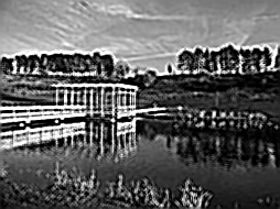
|
| The Original Image |
→
| 0 | 1 | 2 | 1 | 0 |
| 1 | 2 | 3 | 2 | 1 |
| 2 | 3 | 4 | 3 | 2 |
| 1 | 2 | 3 | 2 | 1 |
| 0 | 1 | 2 | 1 | 0 |
| Filter | ||||
→

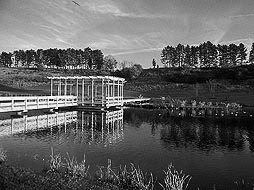
|
| The Blurred Image |
|
→ |
|
→ |
|
||||||||||||||||||||||||||||||||||
|
→ |
|
||||||||||||||||||||||||||||||||||||||||||||||||||||||||||||
| A=filter matrix, x=original image, y=filtered image |
| Ax=y |
| A-1y=x |
|
→ |
|
→ |
|
||||||||||||||||||||||||||||||||||
|
→ |
Conjugate Gradient Algorithm ~400 iterations, 29 seconds on Athlon 800 target r2 = 0.001 |
→ |
|