Breps are produced with the modeling routines, and are input to the mesh generator.
Abstractly, a brep is an acyclic directed graph. Every node in the graph stands for a face of the brep, and the arcs connect faces to their subfaces. Each node has some information associated to it. The graph is leveled: in other words, it is a directed graph whose nodes are partitioned into levels, such that all arcs from level k must go to level k-1 only, for each k.
The bottom level (level 0) is a description of the vertices of the object (for instance, a representation of their coordinates). The next level is the edges of the object, along with pointers to their endpoints at level 0. In general, the kth level contains descriptions of the faces of the object of dimension k, and contains pointers to dimension k-1.
A brep has two integers associated with it: its embedded dimension, which is the dimension of the space it lies in, and its intrinsic dimension, which is the dimension of the object itself. For instance, a square sitting in the z-coordinate plane of 3-space would have intrinsic dimension = 2 and embedded dimension = 3. The programs use the convention that the empty set has intrinsic dimension = -1.
Each face of the brep (node in the graph) has the following items associated with it:
color,
which is used by the rendering routines.
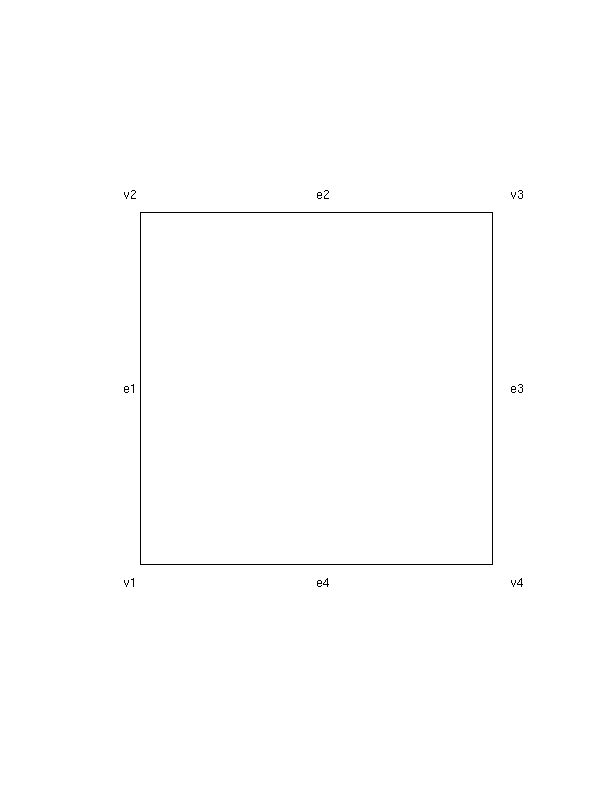
The brep for the square displayed above would have four faces of level 0, four faces of level 1, and one face of level 2. Suppose we refer to the vertex as v1,..,v4 in clockwise order, and the edges as e1,....,e4. Then the children of e1 are (v1,v2). The children of e2 are (v2,v3). The children of e3 are (v3,v4), and the children of e4 are (v1,v4). The square itself has (e1,e2,e3,e4) as children.
Internally, the faces of a brep are numbered consecutively 0, 1, 2, etc. on each level. This internal numbering is used by the gm_addpropval and gmgetf commands, and is also used in the source specification field of simplicial complexes (see below). Except for the fact that the ordering is used to refer to faces, the order of the faces in a level is not significant. Similarly, the order of children in the childlist is unimportant; the order of property-value pairs is unimportant.
Geom_Brep and Geom_SimpComplex, which
is not documented here. The C++ data structures are created while the
routines are running, but they are deleted as soon as the routines
finish so the user never accesses them directly. The mesh generator
has a C++ data structure for breps Mg_Brep
different from the rest of the
routines.
The second representation is called the chunk representation, because in this representation the brep occupies a contiguous chunk of memory. The chunk representation has been designed so that it can be easily unpacked into a C++ data structure and vice versa. The chunks are stored as Matlab arrays. Most of the QMG routines take chunk arguments as inputs and/or return them as outputs.
The actual entries of these arrays are meaningless to Matlab, and the
user should not attempt to directly access or modify individual
entries of a chunk argument (the routines may throw a
segment-violation if presented with an erroneous chunk argument).
Chunk arguments may be saved in files using the Matlab
save command, but they should not be saved with
save -ascii command.
It is permissible to append entries at the end of a chunk array---the unpacking routine will ignore these additional entries.
The third representation of a brep or simplicial complex
is as an Ascii string. This is the only format that can be directly manipulated by
the user. The routine for conversion ascii-to-chunk is called
gm_in
and the inverse conversion is called gm_out.
See below for the details on the Ascii
representation.
There is an accessor routine gmget
to get information from a chunk format brep or simplicial complex. The
routine
gmgetf
returns specific information about an individual brep face.
The only modification routine for chunk breps is gm_addpropval, which adds or modifies a property/value pair
for a face of a brep.
There are no low-level constructor routines for chunk breps. (But
there are high-level geometric constructors, like constructing a
polygon and so on.) The only way in the current system to construct a
brep from scratch is to write a string with an ascii-format brep and
then call gm_in on the string. See the listing of
gmmouse.m for a simple example of this, or
gmcone.m for a more complex example.
Internal boundaries usually serve one of two purposes in a scientific computation: they act as demarcations between separate regions of the domain (for instance, the domain may represent an object that is a composite of several materials) or they act as ``singular'' boundaries, for example, in modeling a region with a slit or crack.
Note that ``holes'' in a domain are not internal boundaries -- they are classified as ordinary boundaries.
Internal boundaries are useful because the mesh generator will respect them in its mesh (i.e. mesh elements will not cross through them). They can also be the site of boundary conditions for the finite element package.
There are two kinds of internal boundaries supported by the QMG package: MTL internal boundaries and SL internal boundaries.
MTL stands for ``multiple top-level.'' This means that the top level
of the brep has multiple entries. (``Top-level'' refers to the top
level of the abstract acyclic graph representation described above.)
The opposite of MTL is STL.
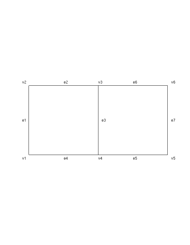
In the square example of a brep
described earlier, we could make a second square at the top level that
shares a common edge, say e_3 with the original square. To accomplish
this, we need two additional vertices v_5 and v_6, three new edges
e_5=(v4,v5), e_6=(v3,v6), and e7=(v5,v6), and one additional
top-level brep whose children are (e3,e5,e6,e7). Thus, there are
two distinct squares at the top level of the brep which have common
descendants. Now e3 acts as an internal
boundary for the overall ensemble of breps at the top level.
MTL internal boundaries are constructed with the
gmsplit routine.
An SL internal boundary corresponds to a ``slit.''
An SL internal boundary behaves in most contexts like a child in
the childlist of a face that is repeated twice (and hence acts like a
slit). In fact, SL internal boundaries are not stored as double
entries in the childlist but are stored as a separate field of the
face. SL internal boundaries are created with the
gmsubtract routine,
From the geometric point of view, SL internal boundaries are more general than MTL internal boundaries, i.e., any internal boundary that can be described as an MTL internal boundary can also be described as an SL internal boundary. The above example of two squares could be represented as follows At the top level would be one six-sided polygon whose children are (e1,e2,e4,e5,e6,e7) and has (e3) listed as an SL internal boundary. SL internal boundaries are more general because they can be used for internal boundaries that cut only partway through the domain.
Even though SL boundaries are more general, MTL internal boundaries are preferable in the case that the internal boundaries represent demarcations between different zones of the domain. In the presence of MTL internal boundaries, the mesh generator will label interior nodes that it generates with the top-level face in which they lie (i.e., the label indicates which ``side'' of the MTL internal boundary the node lies on). See the description of source specifications below. The finite element program can take advantage of the labels during matrix assembly because it can use different functions to compute conductivity and source terms for the two sides of the MTL internal boundary.
In the case of an SL boundary, there is no concept of one ``side'' of the internal boundary versus the other since an SL boundary may cut only partway through the domain. Thus, all interior nodes have the same label. The conductivities can still vary as an SL internal boundary is crossed, but now the function that computes conductivities will have to use the position of the node in some kind of geometric computation of its own to figure out the conductivity for each mesh element.
The mesh generator will produce a single ``layer'' of nodes along either an SL or MTL internal boundary. In some applications a double-layer of nodes is desirable, but this is not currently supported.
This definition implies that the brep faces are always bounded, which is the case for the current system. There is no way to represent unbounded sets.
For example, in the case of a one-dimensional face, the above properties imply that it has an even number of boundary vertices, and all its boundary vertices are colinear. The ray-shooting definition of its geometric set is equivalent to the following simpler definition. The geometric set is the union of the line segments marked off by consecutive pairs of points along the line. Most commonly a one-dimensional face has exactly two children, in which case its geometric set is a single segment. There is no way to represent rays or infinite lines in the current version of QMG.
The remaining correctness properties of breps are:
The mesh generator requires certain additional properties of the breps it triangulates.
As with a brep, a simplicial complex has two integers associated with it, the embedded dimension and the intrinsic dimension. A simplicial complex is specified by three arrays. The first array is the list of vertex coordinates. This array has a number of rows equal to the number of vertices, and a number of columns equal to the embedded dimension of the complex. The entries in the array are double-precision floating point numbers.
The second array is a list of simplices. The number of rows in this
array is the number of simplices and the number of columns is the
intrinsic dimension plus one. The entries of this array are
nonnegative integers that refer to the vertices (i.e., to row numbers
in the coordinate array). These vertex indices start at 0 so you may
have to increment them by 1 if you retrieve them with
gmget(scomplex,'Simplices') in Matlab.
The geometric set associated with a simplex is defined to be the convex hull of its vertices.
The third array is a list of specifications of a brep face in the in the brep from which the complex was generated (the ``source specification''). This specification consists of two integers; the first integer is the level of the face and the second integer is the position within the level (numbered 0,1,2, etc.)
Notice that this array specifies the brep face, but does not actually specify which brep gave rise to the mesh generator. In the current version of QMG it is the user's responsibility to keep track of which brep gave rise to which simplicial complex.
The correctness properties of a simplicial complex are:
If a simplicial complex is specified in conjunction with a brep (i.e., it is a putative triangulation of the brep), it must satisfy the following additional correctness conditions.
gmchecktri An important property of a simplex is its aspect ratio. The aspect ratio of a simplex can be defined in several ways which are all equivalent up to constant multiples. In the QMG package, aspect ratio is defined as the ratio of the length of the longest edge of the simplex divided by its shortest altitude.
Small aspect ratios are desirable because large aspect ratios cause a loss of accuracy in the finite element approximation, and can also lead to condition number problems for the assembled stiffness matrix.
The delimiters for crossproducts are <...>. The delimiters for a list are (...). That is, the sequence of items enclosed in <...> are all of different types, and the type of each entry is known in advance from its position in the sequence. The items enclosed in (...) are all of the same type, and the number of items enclosed in (...) is not necessarily determined in advance syntactically.
The idea of representing a brep as recursively nested crossproducts was suggested by S. Allen.
The rules for an Ascii representation may be defined by the following production rules.
brep or
simpcomplex.
nil .
nil
terminates the recursion; the depth of the nesting before nil
is encountered must agree with the intrinsic_dim specification above.
This documentation is written by Stephen A. Vavasis and is copyright (c) 1995 by Cornell University. Permission to reproduce this documentation is granted provided this notice remains attached. There is no warranty of any kind on this software or its documentation. See the accompanying file 'Copyright' for a full statement of the copyright.
geom.html,v 1.1.1.1 1995/05/05 01:15:54 vavasis Exp
Stephen A. Vavasis, Computer Science Department, Cornell University, Ithaca, NY 14853, vavasis@cs.cornell.edu