Chapter 9
Exchange Networks
In this chapter, we will consider a generalized form of matching markets, referred to as exchange networks. Roughly speaking, rather than just considering bipartite graphs where the left nodes are buyers and the right nodes are items/sellers, we will now consider exchanges over arbitrary networks. We first describe the problem and then relate it back to matching markets.
9.1 Definition of an Exchange Network
Assume we have an undirected graph with nodes; the nodes in this graph represent the players, and an edge between two players means that the players may perform “an exchange” with each other. Each edge is associated with some amount that can be split between its endpoints if an exchange between the endpoints takes place—think of this value as the value of a potential partnership between the endpoints. Nodes can participate in at most one exchange (i.e., they form exclusive partnerships); in other words, the partnerships form a matching in . The outcome of such an exchange network is thus a matching in , and assignments of values to players representing the players’ share of the value of the partnership they (potentially) participate in:
Definition 9.1. An exchange network is a pair , where is a graph and is a function. An outcome of an exchange network is a pair where:
To see how this notion captures a matching market, consider a bipartite —the “left nodes” correspond to buyers and the “right nodes” correspond to the items; the value of an edge between a buyer and an item is simply the value player has for the item . The exclusive partnership condition here models the fact that players only get at most one item, and each item can only be sold to a single player. When the price for an item has been set, and the item gets sold to some buyer , player ’s value for item , gets split between and the seller— gets allocated to the seller and gets allocated to the buyer .
But exchange networks can capture significantly more general strategic interactions, even if is bipartite—we no longer need to view the nodes as “buyers” and “items/sellers,” but rather just as individuals in a social network that engage in some form of exclusive partnerships. In particular, we can now see how some nodes in the social network are “more powerful” than others (due to the network structure), in the sense that they will get a “better deal” in the partnerships they establish. Indeed, such interactions have been empirically studied in the sociological field of “network exchange theory” [Wil99].
To do this, we first need to have a way to generalize the notion of a market equilibrium to exchange networks. The notion of a stable outcome does this.
9.2 Stable Outcomes
We call an outcome stable if no node can improve its allocated amount by establishing a new partnership with some node such that (a) is strictly better off with than in its current allocation, and (b) receives at least as much as it does in its current allocation. Intuitively, if such a pair of nodes exists (i.e., the outcome is unstable), then we would expect to break its current partnership and propose a new partnership to which would accept.1 A mathematically cleaner way of saying the same thing is to require that for every pair of nodes , their currently allocated combined amount, , is at least as large as the value of their potential partnership, : if , then and can, for instance, form a new partnership with the division and (one of them rounded upward and the other downward), where is the surplus on the edge. Since the surplus is positive, at least one of them will be better off and the other at least as well off.
Definition 9.2. Given an exchange network , we call an outcome unstable if there exists a pair of nodes in such that , but (i.e., the edge has a positive surplus). If is not unstable, we call it stable.
In other words, an outcome is stable if and only if all edges have a surplus of 0. Let us now show that this notion indeed generalizes that of a market equilibrium. First, we need to formalize the correspondence between matching markets and exchange networks:
- Given a matching market , we say that is the exchange network corresponding to if (a) is the complete bipartite graph over , and (b) .
- Given an exchange network where is a bipartite graph, we say that is the matching market corresponding to where if , and otherwise.
We now have the following claim.
Claim 9.1. Let be a matching market and let be the exchange network corresponding to . Or, conversely, let be an exchange network where is bipartite, and let be the matching market corresponding to it. Consider any prices , any matching in , and any division function such that:
- if ;
- if and ;
- otherwise.
Then is a market equilibrium in if and only if is a stable outcome in .
Proof. We separately prove each direction.
The “only-if” direction: Assume for contradiction that is a market equilibrium in , but is not stable in —that is, there exists some unmatched buyer–item pair such that . By our construction of , this means that
Thus, , which means that would strictly prefer to buy item at its current price (to buying item that it currently is getting), which contradicts the market equilibrium property of .
The “if” direction: Conversely, assume for contradiction that is stable in , but is not a market equilibrium in —that is, there exists some buyer who prefers buying item at price to the item (or lack thereof) to which they currently are assigned. Assume first that is matched to some object . Then, we have that
By the definition of and , the left-hand side equals and the right-hand side equals ; thus, we have
which contradicts the stability property of . Consider, finally, the case that is . Then , but, since prefers to buy , . So
which, again, contradicts the stability property of .
■
Let us point out that, a priori, there is a surprising aspect of Claim 9.1: the notion of a market equilibrium only says that no buyer wishes to switch to some other item—it does not impose any restrictions on the item/seller not wanting to switch to some other buyer (who may be willing to pay more)—yet the notion of stability (when considering the exchange network corresponding to a matching market) treats buyers and sellers symmetrically and requires that neither of them prefer switching to some other partnership. So, why are we getting this “no-deviation” property also for sellers (for free)? The point is that if a seller could propose a partnership to buyer that is better for , that means there is a surplus on the edge, which in turn means that can also propose a partnership to that prefers to its current deal (i.e., there indeed exists some buyer who prefers to switch to some object that they currently are not matched with).
9.3 Existence of Stable Outcomes
A direct application of Claim 9.1, combined with Theorem 8.2 (which states that market equilibria always exist in a matching market), gives an existence theorem for stable outcomes in bipartite graphs.
Theorem 9.1. Any exchange network where is bipartite has a stable outcome. Furthermore, such a stable outcome can be found in polynomial time in the size of and the maximum value of any edge in the graph.
Proof. Observe that the notion of stability does not depend on the names/labels of the nodes in the graph, so we may without loss of generality assume that set of “left nodes” in the bipartite graph are . By Claim 9.1, a stable outcome in exists if and only if there exists a market equilibrium in the matching market corresponding to ; by Theorem 8.2 such equilibria always exists.
■
A natural question is whether stable outcomes exist in all (and not just bipartite) graphs. The answer turns out to be no, even for very simple graphs.
Claim 9.2. There exists an exchange network with three nodes for which no stable outcome can exist.
Proof. Consider a “triangle” with three nodes (i.e., all nodes are connected by an edge), and for every edge , set the value of the edge, to some integer . Assume, for contradiction, that we have a stable outcome in . Since is a triangle, any matching in can contain at most one edge. If contains no edges, for every node , and thus for any pair of edges , , so is not stable. Consider next the case when contains one edge . One of the nodes, say , must have , and the third node must have (since it is unmatched); thus, , which means the outcome is not stable.
■
Note that the triangle example shows that any outcome, in fact, must have some edge with surplus at least . So, if split the surplus evenly (i.e., offers himself and offers to ), both players gain at least by forming this new partnership. This example thus rules out even more relaxed notions of stability where a deviation is only deemed viable if both players are substantially better off than in their current allocation.
9.4 Applications of Stability
Let us now turn to applying the notion of stability to some example graphs. (All of these graphs are bipartite, so we are guaranteed to have stable outcomes.) Consider the graphs in Figure 9.1, and let for every edge ; think of the value as 100 cents. (Several interesting behavioral experiments have been performed to understand exchange networks in a laboratory setting. In these experiments, subjects are given some small example of a social network—such as the examples in Figure 9.1—and are each assigned to a node in the network, and then need to negotiate a split of a dollar with their neighbors, under the exclusive partnership rule.)
- First, look at the leftmost example, consisting of two nodes with a single edge between them. Typically, we would expect the most “fair” outcome to be a 50/50 split of the dollar, but in fact any division is stable, as neither player is able to make a more advantageous deal with another player. (Usually, in behavioral experiments, we do see something close to a 50/50 split; we will shortly return to this point.)
- Next, the second example, with three nodes in a line, has only two stable outcomes. The middle player can choose to partner with or , but in any stable outcome he gets all of the 100 units. Otherwise, if where to partner with, say, and receives less than 100, then the edge has a positive surplus! So we see that here is “infinitely” powerful—due to its network position, it can extract out all the value!
- In the final, rightmost, example, first note that no stable outcome can contain a matching between the middle nodes ; if it did, one of the nodes (without loss of generality, ) would receive an allocation of at most 50, and there would thus be a surplus of at least 50 between this node and its currently unmatched neighbor (i.e., ). From this, we conclude that any stable outcome must match to , and to . However, we cannot say much more than this: any allocations of the 100 units over these two edges with the property that and receive at least 100 combined (such as the ones illustrated in the figure where, in the first example, all players get 50, and, in the second example, and both take 100) will be stable.
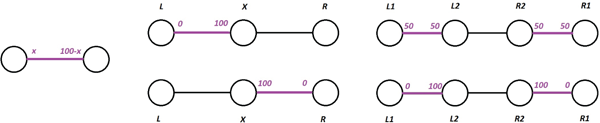
Figure 9.1: Some basic examples of exchange network games, with stable outcomes indicated in purple.
Cut-off thresholds: Rejecting unfair deals An important realization from these examples is that nodes on the “ends” of the lines—that is, nodes that are connected to only one other node—have basically no bargaining power; as they have no alternative options, they are forced to take whatever their single prospective partner offers them! However, in real life, even such isolated nodes have some small amount of power. To better understand the issue, consider the following simple game referred to as the ultimatum game:
- We have two players, and .
- begins by proposing any split of one dollar between himself and , as long as is getting at least 1 cent.
- can either accept the split and take the money he is assigned by , or reject the split, in which case both and get nothing.
One might think that splitting the dollar 50/50 would be an equilibrium of this game. But in fact, it is not, since can always deviate by increasing his cut of the split. In fact, the only PNE of this game is for to propose that he takes the whole pot (99 cents) and for to accept (since accepting is strictly dominant for , and then best responds by taking the whole pot). This is clearly unrealistic—nobody would accept such an unfair deal in real life! Typically, there is some “cutoff threshold” under which an actual person would find the split to be offensive and refuse it, even if it means that they lose a small amount of money. (In fact, in behavioral experiments, this cut-off threshold has been found to be cultural and to depend on several other factors—for instance, a recent study shows that people typically have a higher cut-off threshold when drunk [MKA14].)
To capture this phenomena in the network exchange setting, we can, given some “actual” exchange network, consider (and analyze) an enlarged “mental-experiment” exchange network where each node gets assigned a new “moon” node connected only to , where the edge has a value equal to ’s cut-off threshold; see Figure 9.2. In this moon-enlarged network, no node would ever accept a partnership where they earn less than , since then they would just partner with “their moon” .
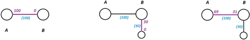
Figure 9.2: Left: A simple two-node network: can propose an arbitrarily unfair split (e.g., to and to ) of the edge weight . Middle: We introduce a “moon” node for with edge weight 30 to model their refusal to accept any deal where they receive less than 30. In this case, will prefer to get matched with their “moon” instead of accepting ’s split from the figure on the left. Right: If proposes a favorable split (in this case, 31), then will accept it.
9.5 Balanced Outcomes
As seen in even the simple two-node example, where essentially any outcome was stable, stability does not always provide enough predictive power. As such, it would be desirable to have a stronger notion of stability that provides more fine-grained predictions about what outcomes one ought to expect.
Nash bargaining Let us first consider the simple example of a two-node graph. Here, we would expect to see an even split between the players.2 This is arguably the “fair” outcome in this simply situation.
But how can we generalize this notion to more complicated graphs? To motivate the definition, consider again a simple two-node network with players and and where the value of edge between them is 1, but, now, let us also assume that has some “outside option” such that he can choose to not match with and still earn some utility ; similarly, let have an outside option, which guarantees him utility . Let denote the surplus that the two players jointly earn from bargaining with one another instead of taking their outside options. Clearly, will never accept any offer that gives him less than , and will never accept any offer where he earns less than . So, effectively, they are now negotiating over how their surplus should be split; effectively, this brings us back to the simple two-node example, where we would expect the surplus to be split evenly.
So should receive (possibly rounded), and should receive (possibly rounded); this amounts to a proper split of that is similarly attractive (except for the possible rounding) to both players given their outside options. John Nash, in his paper on bargaining [Nas50a], indeed suggests that this is the “fair” way to set prices in such a bargaining situation.
Defining balanced outcomes We now rely on the Nash bargaining solution to obtain a strong notion of stability for general exchange networks; we say that an outcome is balanced if, for each edge in the matching, the division corresponds to the Nash bargaining solution wherein each node’s “outside options” are defined by the divisions in the rest of the network—namely, the outside option of a node is defined to be , that is, the maximum value it can earn by making an acceptable offer to some player besides the one it is currently matched with. Note that any balanced outcome clearly also is stable: each node clearly gets at least as much as its outside option, which is what the notion of stability requires.
Revisiting the examples We can now revisit the simple line networks considered in Figure 9.1; for each network, we now have a unique balanced outcome. In the leftmost graph, by definition, the balanced outcome is a 50/50 split. In the second graph, still gets the full 100 units (as this was the only stable outcome, and as such can also be the only balanced outcome). The most interesting case is the rightmost graph. As argued before, there is not stable matching where the middle nodes get matched, and thus they cannot get matched in a balanced outcome either. Note, however, that the middle nodes still have the option of matching with each other and thus have an outside option, whereas the exterior nodes do not (i.e., their outside option is 0). Let denote the respective divisions in some balanced outcome. Since ’s outside option is , and outside option is 0, by balance we have that
By the same argument, we have that
Solving this linear equation yields the solution ; we conclude that . So, as expected, the interior nodes can leverage the fact that they have better “outside options” to get a better deal (i.e., of the 100 units, whereas the the exterior nodes are only getting ). See Figure 9.3 for a summary.
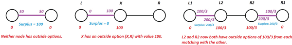
Figure 9.3: Returning to the examples in Figure 9.1, we can analyze the balanced states of each of these by considering each node’s outside options. Outside options are indicated in red, surpluses in blue, and the balanced matchings and splits in purple.
Balanced outcomes indeed provide good predictions of how human players will actually split money in behavioral experiments, not only in the case of a two-node network, but also in more general networks (such as the line networks considered). Additionally, a result by Kleinberg and Tardos [KT08] shows that every exchange network that has a stable outcome also has such an outcome that is balanced; this result, however, is outside the scope of this course.
Notes
Exchange networks for bipartite graphs were first considered by Shapley and Shubik [SS71]; the notion of stability is a special case of the notion of the core introduced by Gillies [Gil59] and studied for exchange networks in [SS71]. As far as we know, exchange networks in general graphs were first considered in [KT08]. The notion of a balanced outcome first appeared in [Roc84, CY92] but the term “balanced” was first coined in [KT08]; as mentioned, the Nash bargaining outcome was first studied in Nash’s paper [Nas50a].
Theorem 9.1 was first proven in [SS71] and a generalized version of it appears in [KT08]; both these proofs rely on heavier machinery (solving linear/dynamic programs). Our proof (relying on the connection between exchange networks and matching markets) is new as far as we know.
Finally, see [EK10, Wil99] for further discussion of behavioral experiments studying exchange networks.
1If amounts are infinitely divisible, can always offer a deal that strictly increases also ’s allocated amount (by some small ), while still ensuring that is strictly better off—this is why we expect to also want to break its current partnership.
2This may not always be the case; for instance, in situations where one of the players inherently has more “social power” (e.g., the left node is the boss of the right node), we would expect to see an uneven split. Again, this phenomena can be captured by relying on the moon-augmented network mentioned above, where the player with more inherent social power gets a “bigger moon.”