SNS Staged Simulator : Overview

We have created the SNS Staged Simulator by applying staging to ns2, a commonly used and well-understood simulator typical of the current state of the art in wireless network simulation. In ns2 the wireless physical layer and mobility models are the largest consumers of processing time in common simulation scenarios. These computations pose the most significant bottlenecks to efficiency and scale. Consequently, we have initially focused on staging computations related to node mobility and the wireless physical layer.

Under typical wireless mobility and physical models, simulators must perform numerous calculations when a packet is transmitted in order to ultimately determine which nodes will receive the packet. These calculations depend strongly on the positions of sending and receiving nodes, packet transmission and reception signal strength thresholds, geography, and radio and antenna models. Consequently, in wireless simulation, neighborhood calculations are fundamental, frequent and expensive.

Mobility computations are an especially challenging domain in which to implement staging, because inputs are dynamically varying and time-dependent. Identical inputs to high-level computations are rarely found within a single run of a simulator, or across multiple similar runs. In addition, the monolithic structure of typical implementations obscures any redundant computations performed at runtime.

Staging in SNS

We incrementally describe four different applications of staging to ns2, each employing a different approach to eliminating redundant computation. The first is an example of decomposing a computation via currying and reusing common intermediate results across events. The second demonstrates the use of upper and lower bounds, or auxiliary results, to enlarge the overlap in computation across events. The third optimization illustrates the use of time-shifting as a staging technique, and the final one demonstrates inter-simulation staging by reusing results across multiple similar runs of the simulator. A surprising result is that the final staged simulator looks nothing like the initial simulator implementation, and achieves a dramatic, qualitative improvement in both performance and scale.

Currying: Grid-based Neighborhood Computation

As an initial, elementary application of staging, we first restructure the neighborhood set computation using a well-known grid-based approach. This computation determines the set of nodes within range of a transmitting node, and hence the nodes that must receive a copy of each packet transmitted by the node. This restructuring is intended to expose the redundancy between and within calls to the neighborhood computation.

	Figure 1: Grid-based neighborhood computation data structure with either fine or coarse-grained grid granularity. The source node at center is transmitting with radius shown. Examined grid bins are shaded, and linked lists indicated by arrows.

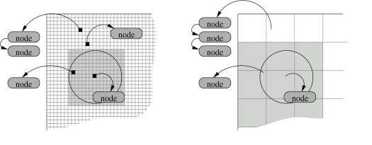
A first example of staging can be seen in a well-known and straightforward grid-based neighborhood computation approach, where we reuse previously computed transmission results for nodes that are close by in distance within a single computation, and expose and reuse partial results between packet transmissions. Grid-based neighborhood computation first divides the coordinate space into a grid of buckets, with each bucket holding a list of nodes positioned within the corresponding grid rectangle. The geographic partitioning and node lists are shown in Figure 1. This partial information about node positions can then be used to quickly determine if a group of nodes falls entirely outside the possible transmission range of a node, thereby eliminating the need to perform individual calculations for each node. Nodes in the remaining buckets, which may or may not be in range, are checked individually as before.

Grid-based neighborhood computation can be classified as staging in two distinct ways. First, the computation is decomposed into two parts, where the first updates the grid if nodes have moved, and the second uses the updated grid to obtain a precise result. The grid data structure is shared across all computations, and updated whenever needed, either lazily, just before a packet transmission, or continually as nodes move. The second use of staging occurs within a single computation. By grouping nearby nodes into grid buckets, a single distance computation or estimate can be used in place of many individual computations. The benefits of grid-based computation stem from reducing the number of nodes examined on each packet transmission, and from sharing grid maintenance across all packet transmissions.

Auxiliary Results: Neighborhood Caching

The grid-based approach provides a base to which we can successively apply additional staging. Variations on the grid approach allow more advanced applications of staging using auxiliary results to reduce redundancy in computation across packet transmissions. In common simulation scenarios, inter-packet spacing is very short in comparison to the speed at which nodes move. Depending on node mobility and traffic patterns, many hundreds or thousands of packets may be transmitted from a single node before nodes move a significant distance. That is, we should expect the inputs to, and hence the results of, the grid-based neighborhood computation for a node to be reusable across many packet transmissions.

	Figure 2: Neighborhood Cache Entry Structure for Node at Center, Showing Transmission Radius r, Δ r = 2 smax Δ t, and Linked Lists (Arrows) for Sets Ninner and Nouter

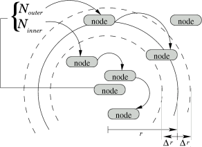
Since node positions will vary slightly, we should not expect the neighborhood set to be identical to the set computed during the previous packet transmission. However, nodes that were sufficiently far from the sender during the previous transmission will still be out of range of the sender, and nodes that were sufficiently close will still be in range. Computing this additional information at the time of packet transmission is efficient, and this auxiliary data can later serve to quickly eliminate many nodes from consideration in subsequent transmissions. These conservative upper- and lower-bounds on the neighborhood set will remain valid for some time after they are computed, depending on the amount of node mobility and the tightness of the bounds, so we can efficiently check if the saved results are reusable. We therefore restructure the neighborhood set computation to first compute an bounds on the result, with a known expiration time, then refine this bound during each packet transmission into an exact result. After restructuring, a straightforward application of function caching is used to cache and reuse the common auxiliary results, the upper- and lower-bounds, across many packet transmissions.

This restructuring exposes one additional parameter, Δ t, to control the caching policy. This parameter fixes the desired epoch duration for which the bound on the neighborhood set will be valid. If s_max is the maximum possible node speed in the movement scenario, then the maximum change in distance between two nodes in an epoch is just Δ r = 2 s_max Δ t. If two nodes are within distance r - Δ r at some time, then they will remain within range r for Δ t seconds into the future. Consequently, the precise position of nodes beyond distance r + Δ r need not be computed at all for Δ t seconds into the future. Thus, neighborhood caching further reduces the number of nodes that need to be examined on every packet transmission, since only nodes in the annulus around the sender could have changed status since the last packet transmission.

We maintain a cache to capture this upper bound on the neighborhood set of each node. At most one cache entry is maintained for each node in the network. A cache entry, illustrated in Figure 2, is composed of an expiration time and two sets, N_inner and N_outer, containing lists of the nodes within a ball of radius r - Δ r and those in the annulus with radii r ± Δ r. During packet transmission, the cache manager computes the set of nodes within range of a given node by first looking for a valid cache entry. Finding an entry that has not yet expired, it can immediately consider all nodes in the list N_inner to be within range. The second list N_outer is then scanned, and each node found to be within range is appended to the final result. At the same time, it can cheaply but conservatively update the lists, moving some nodes from N_outer to N_inner and eliminating others from N_outer entirely. If, on the other hand, no cache entry is found during packet transmission, the cache manager consults the underlying grid and constructs a cache entry with expiration Δ t seconds into the future.

In the above caching scheme, there is some additional overhead during cache misses, when computing N_outer, since a larger radius is considered than previously necessary. This overhead is controlled directly with the parameter Δ t, which fixes the longevity and the accuracy of cache entries. In addition, there is overhead associated with scanning the list of nodes in N_outer during each cache hit, but this is also limited by appropriately choosing the Δ t parameter.

Time-shifting: Perfect Caching

We can expand the overlap in computation by looking for other redundancies than that addressed by neighborhood caching. Here, we target the overlap in computation when two nearby nodes each independently compute their neighborhood sets. The intuition is that nearby nodes transmitting at the same time will have very similar, if not identical neighbors.

There is a large overlap in computation when constructing multiple cache entries independently. In the worst case, each pair of nodes will be considered twice, as the receiver of a packet does not take advantage of the distance computed by the sender. This is especially acute in light of the rapid sequences of packet exchanges between a pair of nodes, which are common in wireless MAC and network protocols. It is unlikely that two nodes will transmit packets at identical times. However, neighborhood cache entries can be constructed at any time, so we can use time-shifting to address this redundancy by reordering the creation of cache entries.

A staged simulation approach, which we term perfect caching, eliminates this redundancy by precomputing all cache entries simultaneously. This approach maintains the same data-structures as neighborhood caching. But, rather than calculating cache entries on-demand, it precomputes all cache entries at the beginning of every Δ t epoch. All normal queries for neighborhood information are then guaranteed to be satisfied from the cache. There are two potential advantages to batching computation in this way. First, by grouping all accesses to the mobility data-structures, the simulator might achieve higher memory locality and improved working set sizes. And second, we can implement a more efficient algorithm that simultaneously computes all of the cache entries together, rather than individual computations for each entry. Specifically, the positions of all nodes can be updated only once per epoch, just before the single computation, and each pair of nodes need be examined at most once per epoch, rather than twice.

The overhead of this technique is a scheduled event during each Δ t epoch. Also, perfect caching may introduce additional, wasted computation if some nodes do not send packets during an epoch, and thus do not use their cache entries. In a sparse or quiet network, perfect caching might construct more entries than needed during the simulation. This potential for wasted work can be addressed by appropriately choosing the Δ t epoch parameter.

The underlying grid is normally maintained during each epoch as nodes move about the geography. At each time a node moves across a grid boundary, an event must be scheduled to update the affected grid cells. In many networks this maintenance can be very expensive. However, the perfect caching approach accesses the underlying grid only once per epoch, opening the possibility that the grid might be re-created from scratch once per epoch, rather than maintained and updated from one epoch to the next. Staging introduces a new trade-off in choice of maintenance versus re-creation. This trade-off depends on the size of the network, which impacts the cost of grid re-creation, and the amount of mobility, which impacts the cost of maintenance.

Inter-simulation Reuse: On-disk Caching

A final inter-simulation staging application improves on perfect caching and demonstrates how staging can be applied across multiple similar runs of the simulator. Inter-simulation staging expands the scope of caching and reuse to span multiple runs of the simulator by using the disk as a persistent cache. In the first run of the simulator, cache entries are generated and expire exactly as in intra-simulation staging. As cache entries expire, however, they are written to disk for use in later simulator runs. Disk access can be done efficiently in the background by introducing a moving window and a worker thread. The moving window covers cache entries that have expired, but have not yet been written to disk. The worker thread, operating entirely in the background, can spool these entries to disk, then expunge them from the cache. Subsequent runs of the simulator perform a complimentary procedure. Here, the worker thread prefetches cache entries in the background, saving them into a sliding window just ahead of the simulation clock. The simulator can then use these cache entries directly until they expire and are immediately expunged. Again, all disk accesses are performed in the background.

We apply inter-simulation staging to the perfect caching scheme described above. This takes advantage of common simulator usage, where a batch of simulator runs often share a single mobility scenario. In this case, perfect caching will perform identical work during each simulation run, since cache entries are computed at pre-chosen times independent of the network load or other simulator parameters. The first run of the simulator saves all neighborhood cache entries to disk, and the second and subsequent runs avoid recomputing these entries by reading the results directly from disk.

The amount of computation saved in this manner is potentially significant. The intra-simulation examples above, while reducing the amount of computation during packet transmission, also add some additional work to maintain or re-create the grid for use during cache misses. In particular, many grid-crossing events might be scheduled in the event queue, leading to more work in the event scheduler and dispatcher. This application of inter-simulation staging builds on the intra-simulation staging techniques by reducing the number of scheduled events generated by the grid manager and the cost of constructing neighborhood cache entries in the perfect caching scheme. Surprisingly, in the second and subsequent runs of the simulator we can eliminate the underlying grid entirely, as well as all the work for constructing cache entries, since all requests will be satisfied by cache entries read from disk.