2.3 Local Minimization

2.3.1 The weaknesses of local minimization

Remember from last lecture the definition of local minimization:

1. Start with a guess for F, for example with G.
2. Pick and F' near F.
3. If E(F')<E(F) then F:= F'
4. Go to step 2

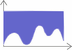
Local minimization will find a local minimum, but we are actually interested in the global minimum.

Example:

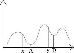
In 1 dimension, the situation may look like the following:

You will probably find the global minimum A if you start the search at point x, but if you start at point y, you are more likely to find the local minimum B.

In general, the global minimum is hardly ever found in practice. Note also that local minimization has difficulties at inflection points (which correspond to saddle points in higher dimensions) and at plateaus, because these areas of the function surface look locally as if there were no further improvement possible.

Most energy functions we will be dealing with have many local minima, but there is a class of functions that has only one minimum. Functions with this property are called convex and local minimization will successfully find the global minimum for these functions.

2.3.2 Convex functions

We mentioned already that convex functions have only one minimum, but there is also a second, more formal definition:

A shape is convex iff . A function is convex if the area above the function curve, the so-called upper envelope is a convex shape.

In plain English, this definitions means that for any two points x and y inside the shape, the line in between the two points is also inside the shape.You can easily see from that definitions why convex functions can have only one minimum.

The property of convexity is actually quite important because it makes optimization tractable.

	local	global
Convex	"easy"	"easy"
Non-convex	"easy"	"hard", req. exp. time

Unfortunately, computer vision problems lead very often to global optimization problems of non-convex energy functions and many of the algorithms of optimization theory cannot be used. One of these problems is the stereo problem which we introduce next, first intuitively and then by its formulization as regularization problem. In the subsequent lessons we will then develop a stochastic method for global minimization.

2.4 The Stereo Problem

2.4.1 Informal definition

Consider the following situation of two cameras that are simultaneously taking images of a scene.

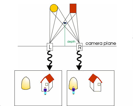
Notice that by going from the left image to the right image, the world 'moves' to the left. You can easily verify that by holding your thumb in front of your face and looking at it first with only your left eye and then with your right eye. The amount of shift of a point in the left image (in terms of coordinate distances) to the corresponding point in the right image is called its disparity. Notice also that near objects have high disparity whereas objects that are far away do not move much. That means that disparity is inversely proportional to depth, i.e. the distance of a point in the real world as measured orthogonal to the camera plane.

Therefore, we can actually reconstruct the distance of the objects in the scene from the camera up to a scaling factor by determining the disparity value for each point in the image. The stereo problem is just the computation of this disparity map.

Humans use stereo vision to determine the depth of objects approximately within grasping reach, and if we could compute the disparities fast, it would be useful for the sensor-motoric control of grasping robot arms as well ¹ .

2.4.2 Formulation as a regularization problem

We make the following assumptions:

1. Depth and disparity vary smoothly over the image.
2. Corresponding pixels have the same intensity.

Assumption 1 is obviously not true: depth varies quickly at object boundaries. It is however true that this assumption holds for most points. Assumption 2 holds only for a perfect image formation process without noise and cameras without gain or bias(gain is a multiplicative factor of the intensities and bias an additive factor). Even two cameras of the same brand and model usually have different gain and bias, but we neglect these issues for the moment. We also neglect for now the fact that some points from the left image can be occluded in the right image or that new points can appear in the right image.

Let L(x,y) and R(x,y) be the left and right image, respectively. Let D(x,y) denote the disparity, that is a map of translations such that L(x,y) corresponds to R(x-D(x,y),y). Without noise and occlusion, L(x,y) would equal R(x-D(x,y),y). The minus sign stems from the fact that 'the world moves left' when going from the left image to the right image. Now the energy function becomes

.

The first term, the so-called data term corresponds to the second assumption, while the second term, the smoothness term, corresponds to the first assumption.

The disparity map D that minimizes this energy function is therefore most like the data and also smooth.

Next we will introduce simulated annealing, a stochastic method for solving global optimization problems such as the stereo problem. But before we do so, we have to review the basic elements of probability.

¹Be warned that the grasping-robot-arm-problem is extremely difficult.Even if we could compute depth fast and accurately, we would still be a long way off actually accomplishing the task.