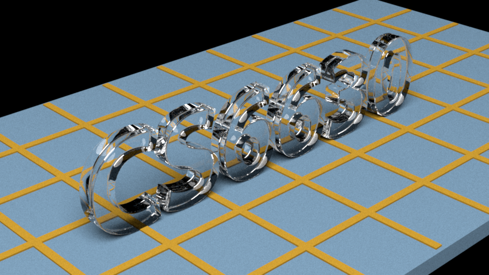
Some text refracting a grid.
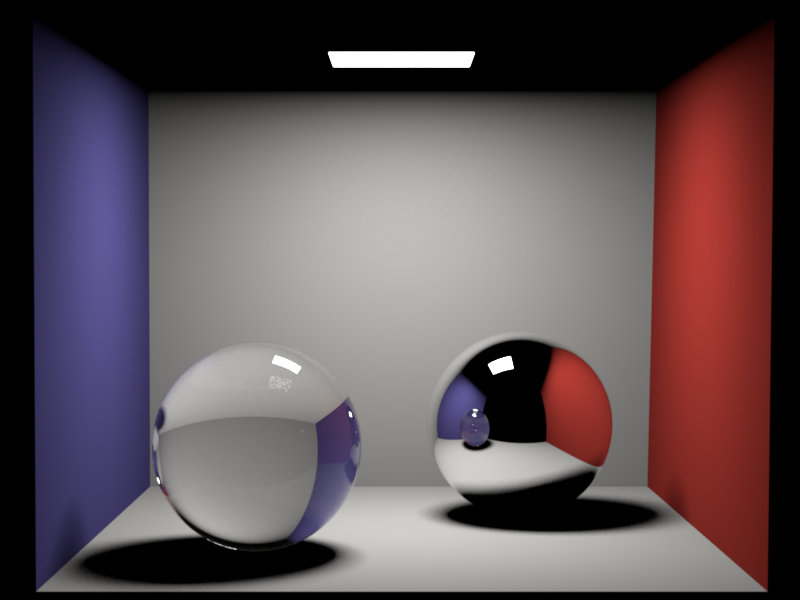
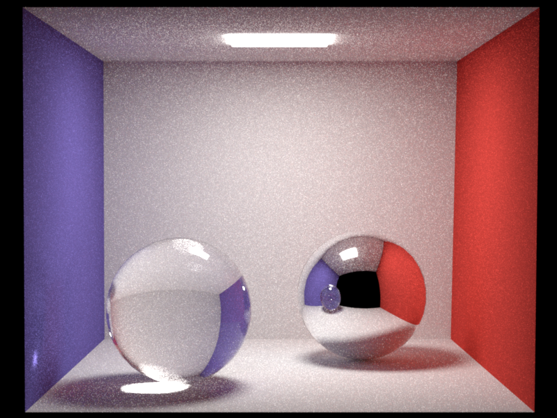
A Cornell box containing glass and metal spheres
This assignment marks the culmination of the sequence of previous assignments. You will build a path tracer that accounts for global illumination to render realistic images featuring interreflection between objects with advanced reflectance models that account for surface roughness.
As usual, begin by importing the latest base code updates into your repository by running
$ git pull upstream master
If there were any concurrent changes to the same file, you may have to perform a merge (see the git tutorials under "Preliminaries" for more information).
Take a look at the file src/mirror.cpp, which defines BSDF
of a perfect mirror based on a Dirac delta function.
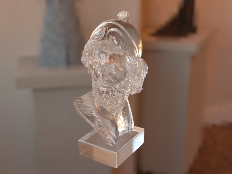
Complete the template in src/dielectric.cpp to implement
the sample() method for a dielectric (i.e. refractive)
BSDF based on Snell's law and the Fresnel equations.
Note that while the mirror sampling code is completely
deterministic, the dielectric BSDF should use the supplied
random sample to choose between a reflection (proportional to the
amount of reflection) and a refraction event (proportional to the
amount of refraction).
One potential gotcha: when we discussed specular BRDFs in class, they
involved a division by a cosine factor to cancel out a corresponding
term from the reflection integral equation. Due to the convention used
by implementations of the BSDF::sample interface (see
include/nori/bsdf.h for details), this division is not
needed in Nori.
Specifically, any BRDFs that require a cosine factor in the reflection
integral should multiply by it in sample(), while specular
materials simply omit this step.
Hint: We already provide you with the implementation of the Fresnel equations fresnel, which you can find in common.h/common.cpp.
Make sure to discuss the relevant technical information about your implementation in the report.
To test out the implementation of dielectrics, extend your direct integrator from the previous assignment into a Whitted-style ray tracer (named after Turner Whitted) that is able to account for specular reflections and refractions.
Modify your direct illumination integrator as follows:
BSDF::isDiffuse()).
In the latter situation, simply fall back to your previous implementation.
The specular case is treated specially: instead of sampling a
position on a light source, invoke the specular surface's BSDF::sample()
method to generate a reflected or refracted direction. This will produce a sampling weight \(c\) and a new direction \(\omega_r\).
Li() method:
\[
L_i(\vc, \omega_c) = \begin{cases}
\frac{1}{0.95}c L_i(\vx, \omega_r),&\text{if $\xi < 0.95$}\\
0,&\text{otherwise}
\end{cases}
\]
This recursion continues for as long as the reflected or refracted rays hit specular surfaces, stopping either when it finds a diffuse surface or when it decides to stop due to Russian Roulette. If it ends at a diffuse surface, the radiance is calculated using the existing direct illumination implementation.
scenes/pathtrace:Please discuss the design choices and relevant technical information about your implementation in the report and include comparisons against our reference renderings.

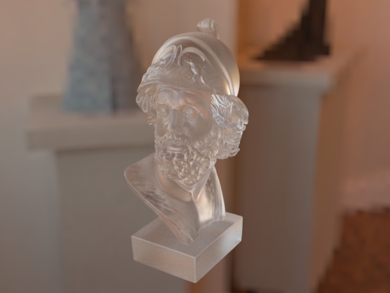
In this part we will extend the rudimentary implementation in microfacet.cpp into a full-fledged reflectance model following the details in [Walter et al. 2007]. This utilizes the sampling techniques for the Beckmann distribution that you implemented in a previous assignment. The process is split into two parts.
The Microfacet BRDF in src/microfacet.cpp will be used to simulate plastic-like materials. It consists of a linear blend between a diffuse BRDF (to simulate a potentially colored reflection from the interior of the material) and a rough dielectric microfacet BRDF (to simulate a non-colored specular reflection from the rough boundary). Implement Microfacet::eval() which evaluates the described microfacet BRDF for a given pair of directions in the local shading coordinate frame:
\[
f_r(\bold{\omega_i},\bold{\omega_o}) = \frac{k_d}{\pi} + {k_s} \frac{D(\bold{\omega_{h}})~
F\left({(\bold{\omega_h} \cdot \bold{\omega_i})}, \eta_{e},\eta_{i}\right)~
G(\bold{\omega_i},\bold{\omega_o},\bold{\omega_{h}})}{4 \cos{\theta_i} \cos{\theta_o}\cos\theta_h}, ~~
\bold{\omega_{h}} = \frac{\left(\bold{\omega_i} + \bold{\omega_o}\right)}{\left|\left|\bold{\omega_i} + \bold{\omega_o}\right|\right|_2}
\]
Here, \(k_d \in [0,1]^3\) is the RGB diffuse reflection coefficient, \(k_s = 1 - \max(k_d)\), \(F\) is the Fresnel reflection coefficient (check common.cpp), \(\eta_e\) is the exterior index of refraction and \(\eta_i\) is the interior index of refraction.
The various \(\cos\theta_k\) cosine factors relate to the angle that the corresponding direction \(\bold{\omega_k}\) makes with the Z axis in the local coordinate system.
The shadowing term uses a rational function approximation provied by Walter et al.:
\[
G(\bold{\omega_i},\bold{\omega_o},\bold{\omega_{h}}) = G_1(\bold{\omega_i},\bold{\omega_{h}})~G_1(\bold{\omega_o},\bold{\omega_{h}}),
\]
\[
G_1(\bold{\omega_v},\bold{\omega_h}) = \chi^+\left(\frac{\bold{\omega_v}\cdot\bold{\omega_h}}{\bold{\omega_v}\cdot\bold{n}}\right)
\begin{cases}
\frac{3.535b+2.181b^2}{1+2.276b+2.577b^2}, & b \lt 1.6, \\
1, & \text{otherwise},
\end{cases} \\
b = (\alpha \tan{\theta_v})^{-1}, ~~
\chi^+(c) =
\begin{cases}
1, & c > 0, \\
0, & c \le 0,
\end{cases} \\
\]
where \(\theta_v\) is the angle between the surface normal \(\bold{n}\)
and the \(\omega_v\) argument of \(G_1\).
The definition for the Beckmann distribution, which is used to model the probability density of normals on a random rough surface, is the same as in Assignment 1: \[ D(\theta, \phi) = \underbrace{\frac{1}{2\pi}}_{\text{azimuthal part}}\ \cdot\ \underbrace{\frac{2 e^{\frac{-\tan^2{\theta}}{\alpha^2}}}{\alpha^2 \cos^3 \theta}}_{\text{longitudinal part}}\!\!\!. \]
In this part you will generate samples according to the following density function: \[ k_s ~ D(\omega_h) ~ J_h + (1-k_s) \frac{\cos{\theta_o}}{\pi} \] where \(\omega_o\) is sampled and \(J_h = (4 (\omega_h \cdot \omega_o))^{-1}\) is the Jacobian of the half direction mapping discussed in class. This can be done using the following sequence of steps:
Warp::squareToBeckmann that you previously implemented in Assignment 3.Once your microfacet material works, your direct integrator should be able to render scenes containing this material in all its modes. However, it's possible that this new BSDF will reveal bugs that were previously not exercised because all BSDFs were diffuse, and you will need to fix those at this point.
Note that you will need to implement both Microfacet::sample() and Microfacet::pdf() to be able to run the following tests.
To validate the correctness of your code:
scenes/pathtrace/tests:The warptestGUI also contains a \(\chi^2\) test for the BRDF model, but this is just to facilitate debugging and visualization; the XML files are the real validation benchmark. Mention in your report if running these tests produces any errors.
scenes/pathtrace:Make sure to discuss the design choices and relevant technical information about your implementation in the report and include comparisons against our reference renderings.
The last three parts of this assignment build three path tracing integrators that generalize the three sampling strategies of the direct illumination integrator from the previous assignment. The first strategy is BSDF sampling, which leads to a path tracer that always extends its path by sampling a direction according to the BSDF and tracing a ray to find the next point.

We will extend the Whitted-style direct illumination algorithm into a full path tracer that fully accounts for indirect illumination. The main difference from the bsdf mode of the direct integrator is that it includes reflected radiance, rather than just emitted radiance, when evaluating the incoming radiance at the shading point.
Create a new "material sampling" path tracer named src/path_mats.cpp that does exactly this. You should use BSDF::sample() to generate new outoing directions at each scattering event. This outgoing direction
is used to estimate both direct and indirect illumination. This corresponds to the algorithm called "Kajiya-style path tracing, version 0.75" in lecture. We recommend that you implement all integrators in this homework using an "iterative" approach with a for-loop compared to the recursive implementation shown in the lecture slides. While the recursive implementation is elegant and corresponds to the idea of a recursive estimator, an iterative approach is more efficient and also generally easier to debug. If you are finding the iterative mode confusing you might find it a helpful exercise to convert your Whitted-style direct integrator to an iterative implementation and verify it computes the same results.
Note: to match the reference renders exactly, you will need to use the following Russian Roulette heuristic for path termination:
continuation probability = min(maximum component of the throughput * eta^2, 0.99)where eta is the product of all \(\eta\) terms encountered along the path, starting with eta = 1.f. Additionally, we recommend to only start doing Russian Roulette after at least three bounces in order to avoid terminating very short paths which can lead to unnecessarily high variance.
scenes/pathtrace:scenes/pathtrace/tests: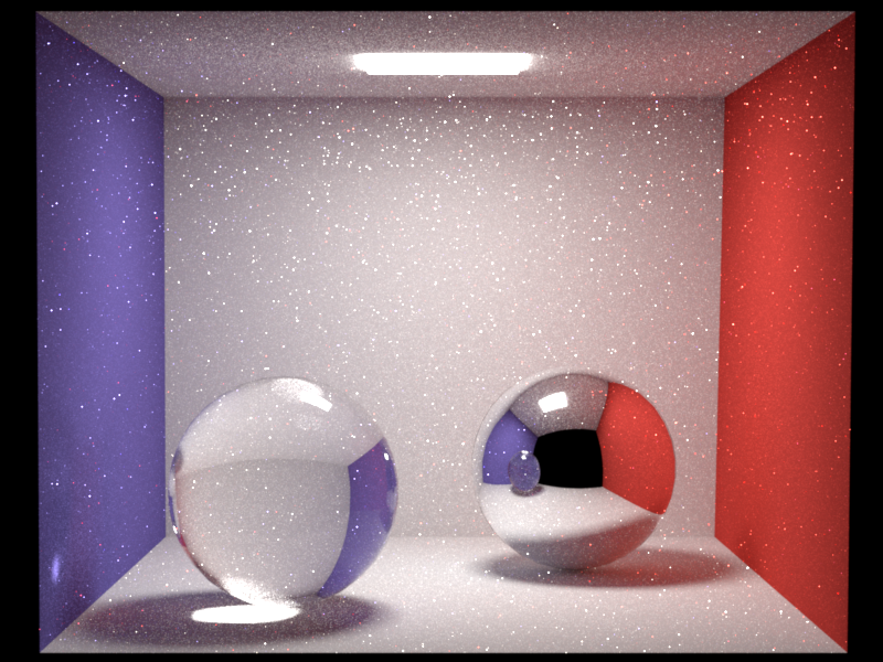
While BSDF sampling alone does work, you will have noticed that it suffers
from high variance in "easy" areas dominated by direct lighting, since its sampling strategy relies on finding the light "by accident." This can be improved by replacing the last bounce with an emitter-sampling estimator just like the one in the previous assignment. We'll implement this in
an "emitter sampling" (ems) path tracer named src/path_ems.cpp (this
corresponds to the algorithm called "Kajiya-style path tracing, version 1.0" discussed
during the lecture).
Starting from path_mats, simply add in the emitter sampling strategy of your direct integrator while taking care to avoid the
"double counting" problem discussed in the lecture.
Note: Different (correct) implementations of emitter sampling will lead to potentially very different noise patterns in the test scenes. If you want to match the reference renders exactly, you will need to (in each iteration) 1) Pick one light source uniformly at random, and 2) Sample one point on the associated mesh uniformly over its surface area.
scenes/pathtrace:The first scene only uses diffuse and specular materials and can be used to test your path tracer if you didn't do part 1 of this assignment yet. The latter two assume that the microfacet model BRDF is ready.
scenes/pathtrace/tests:Make sure to discuss the design choices and relevant technical information about your implementation in the report and include comparisons against our reference renderings.
For this last part you will combine both sampling strategies from the previous tasks into one integrator src/path_mis.cpp that has multiple importance sampling, corresponding to "Kajiya-style path tracing, version 1.0m" from lecture.
You should be able to reuse much of the code from the mis mode of your direct integrator, with the difference that the BSDF sample will continue the path in another iteration of your loop to add contributions from later bounces. Some reminders about the MIS implementation:
BSDF::pdf()) with which the BRDF sampling strategy would hypothetically have sampled the same direction.Remember that the MIS computation is being used to estimate the direct illumination at the point being considered. Since only the BSDF sample is used to continue the path, MIS weights for one shading point should not apply to the contributions of later points along the path (those points will have their own MIS weights based on their own emitter and BSDF samples).
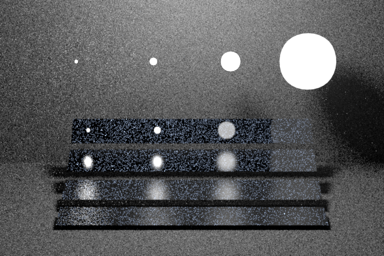
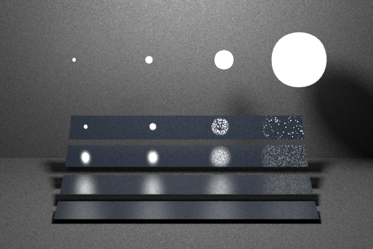
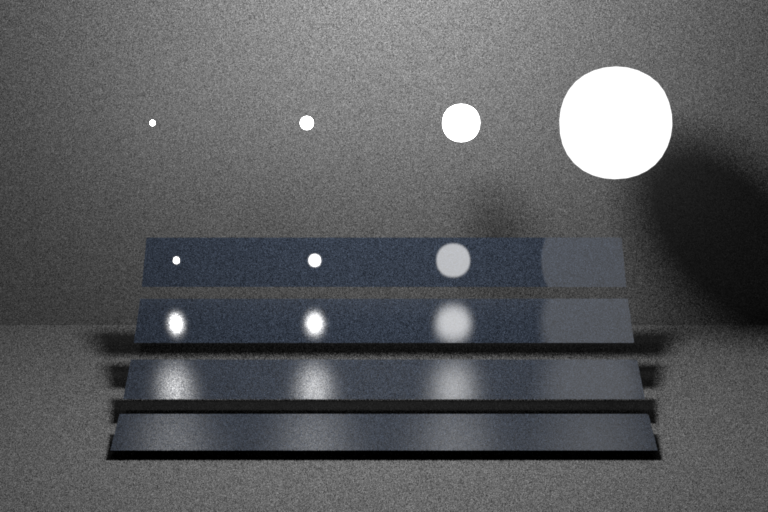
Have fun rendering the various scenes and exploring the performance of the different methods and the effects of scene parameters. The table scene is an example of one where BSDF sampling is a pretty good strategy because the light sources are very big; here MIS does not really do better than BSDF sampling alone. This scene and the glass CS6630 scene show the importance of path tracing in computing shadows of glass objects, which are far too dark if you omit paths from the source through the glass to diffuse surfaces.
scenes/pathtrace:scenes/pathtrace/tests:Build your own artistically appealing scene and include a rendering of it in your report. Use any of the implemented integrators so far—or build something entirely new! Be creative, your renderings may be posted in a gallery on the course website, with your permission. This is a good exercise to get some practice putting together a scene by yourself. This skill will be very useful for creating your scene for the final project.
We recommend using the 3D modeling tool Blender. It can be used to arrange models or to create your own. Feel free to use existing models from websites such as Blendswap. We provide a (rudimentary) Blender plugin (ext/plugin) that can help with some of the steps involved with exporting a scene to the Nori description language, but some manual steps will still be needed to set up integrators, materials, etc.
Please include a short section in the report with your render and credits to any 3D models you used.
For this part your task is to extend the rough dielectric BRDF into a complete BSDF that also accounts for refraction. You will also want to remove the diffuse component as well as the \(k_d\) parameter. Begin by reading the paper Microfacet Models for Refraction through Rough Surfaces by Bruce Walter, Stephen R. Marschner, Hongsong Li, and Kenneth E. Torrance.
To support rough refraction, you implementation will need to randomly choose between the reflection and the refraction component based on the Fresnel coefficient. Follow the instructions in the paper by Walter et al. to add the latter case based on the generalized half-direction vector for refraction.
Our current camera always sends rays a single viewpoint. Real cameras have finite apertures and focusing lenses, which leads to images with a finite depth of focus. Following the PBR book, extend the camera so that it can model a finite-aperture camera and generate renderings that simulate the depth of field of a real camera.