Profile-Guided Code Layout

by Gautam Mekkat October 23, 2019

The goal of this project was to optimize Bril programs with profile-guided function reordering and basic block reordering to improve code locality. I used Bril() to serve as a base for the optimization since it allows for function calls and passing in input via the command line.

Defining Code Locality

Before moving further, it is important to clearly define what "code locality" means. Typically, the goal of code layout optimizations is to improve instruction cache and instruction TLB utilization. When an instruction is loaded into the instruction cache, a block of instructions are loaded into the cache (known as a cache line). To improve cache utilization, we want to minimize the number of times we load into the instruction cache. In other words, we want sequences of instructions that frequently run together to live close together in the code.

That being said, there are many factors that make measuring this metric difficult for this project. Firstly, since Bril is interpreted, we do not load Bril instructions directly into the instruction cache. I considered lowering Bril programs to LLVM using a project 1 extension and then evaluating the lowered program, but that leads into the second problem: I am one person running Bril programs on one machine. The results I find for my machine may not be consistent with other machines, so results would be misleading. Because of this, I use a different metric to measure code locality: instruction pointer jumps. Improving code layout usually decreases the total number of instruction pointer jumps, since frequently executed code lives close together. To introduce the notion of an instruction pointer to the interpreter, I use the index of the currently executing instruction. Every time an instruction is executed, we can compare the current instruction pointer location to the previous location to determine the number of instruction pointer jumps. In other words, we are measuring the distance between the current instruction and the previously executed instruction.

Design

The designs of these optimizations are closely related to the optimizations discussed in "Profile guided code positioning" (1990) by Pettis and Hansen and "Optimizing function placement for large-scale data-center applications" (2017) by Ottoni and Maher. Specifically, the basic block reordering optimization follows the approach laid out the first paper, and the function reordering optimization follows the approach in the second paper. Both optimizations are profile-guided, meaning they use sample inputs to make optimization decisions. Assuming that real-world workloads mirror the sample inputs, we can optimize the code layout for the sample inputs, and this should lead to improved performance on real workloads.

Profiling

The first step in any profile-guided optimization is—perhaps unsurprisingly—profiling. But first, we need to know what kind of data we want to collect when profiling Bril programs. Function reordering relies on weighted directed call graphs, where nodes represent functions, edges represent calls from one function to another, and edge weights are the number of times that call occurred in the sample workload. Similarly, basic block reordering relies on weighted control flow graphs, where edge weights are the number of times the corresponding branch was taken. Therefore, when profiling a Bril program, we would like to keep track of function calls and branches. In addition, to help with evaluation, we will keep track of the total number of instruction pointer jumps.

To build a Bril profiler, I first extended the parser to create an annotated JSON representation of the program. I introduced a new "block" key for every instruction, denoting which basic block each instruction belongs to, and a "line" key, denoting the line number of the instruction (ignoring whitespace) in Bril's JSON representation. In other words, "line" points to the index of the instruction in the program. The first instruction in the first function is 1, the second is 2, and so on. I then extended the interpreter to accept profiling data in the form of a line-separated list of command-line arguments. It then passes each line of the profiling data to the program, tracking function calls and basic block changes. The profiler returns a JSON representation of the weighted call and control flow graphs. The format of the profiling output is shown below.

{
  "call_graph": [
    {
      "from": caller name,
      "to": callee name,
      "count": total number of times called
    },
    ...
  ],
  "basic_block_flows": [
    {
      "from": block label,
      "to": block label,
      "count": total number of times branched,
      "function": function where "from" and "to" blocks live
    },
    ...
  ],
  "total_ip_jumps": total number of instruction pointer jumps
}

To decouple the interpreter from the profiler, I created a new command called brilprofile. It reads Bril programs as JSON from stdin (like brili), but it takes an additional argument, a path to the sample workload. For example, suppose we have a program called fibonacci.bril that takes an integer as a command-line argument. If we have a workload fibonacci.in that contains line-separated integers, we could profile the program by running:

bril2json < fibonacci.bril | brilprofile fibonacci.in

Let's first take a look at how basic block reordering and function reordering are done, and then we'll run through an example from start to end.

Basic Block Reordering

Basic block reordering uses a weighted control flow graph to determine which basic blocks should be close to each other. We want basic blocks that frequently run one after another to live closer together. As a result, it makes sense to co-locate basic blocks that have higher-weighted edges. To do this, I followed a greedy approach introduced by Pettis and Hansen. At a high-level, it works by coalescing basic blocks into chains and ordering these chains to form the new block order. Initially, each basic block belongs to its own chain. We define the source node of a chain as the last node, and the target node as the first node. Note that initially every block is a source and a target. Then, the algorithm works as follows.

Iterate over edges in decreasing order of weight.
During each iteration, if the tail of the edge is a source and the head is a target, then combine the two chains into one chain.
Continue until no more chains can be coalesced.
Order the remaining chains based on frequency of execution. More frequently run chains should be placed higher in the function.

One exception to the above is that the first block in a function must remain the first block in a function since it is the function's entry point. As a result, it must always be a target node, and its chain must be explicitly placed at the top of the function.

Function Reordering

Function reordering uses a weighted call graph to determine an improved function order. The approach is similar to that of basic block reordering. I followed the approach laid out by Ottoni and Maher, with some modifications to account for the limitations of the Bril interpreter. Function reordering works as follows:

For each node, we assign a "hotness" metric, defined as the sum of their incoming edge weights.
Iterate over the nodes in decreasing order of hotness.
During each iteration, determine the node's highest-weight incoming edge, and coalesced the node with the source of the edge.
- Each node has a memory of the order in which nodes are coalesced. For example, if the edge is (a, b), then after coalescing, the new node will record that b is ordered after a.
Continue until no edges remain.

The final node's order is the function order. The difference in this approach compared to the one in the paper is that the paper incorporates page sizes in its ordering. Since we do not have the notion of a page in the Bril interpreter, I just ignore that. The above algorithm is the same as the one in the paper if we assume unlimited page sizes.

An example

To get a better idea of how these optimizations work, let's run through an example from start to end. The following Bril program takes in two command-line arguments a and b, and computes exp(a, b).

multiply a b : int {
  zero: int = const 0;
  one: int = const 1;
  curr: int = id zero;
start:
  b_zero: bool = eq b zero;
  br b_zero end cont;
end:
  ret curr;
cont:
  curr: int = add curr a;
  b: int = sub b one;
  jmp start;
}

main base exp {
  zero: int = const 0;
  one: int = const 1;
  val: int = const 1;
start:
  exp_zero: bool = eq exp zero;
  br exp_zero end cont;
end:
  print val;
  ret;
cont:
  val: int = call multiply val base;
  exp: int = sub exp one;
  jmp start;
}

Below is the workload we will use to profile the program.

Now, if we run brilprofile on the program with the above workload, we will get the following call graph.

The function reordering algorithm will place main before multiply, since main calls multiply.

Below is the basic block graph for main.

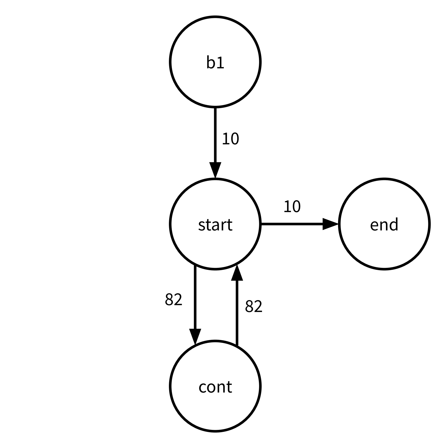
The basic block reordering algorithm will first coalesce start and cont and then prepend b1 to that chain. Since end cannot be added to this chain, it will remain on its own. Combining the chains will lead to a final block order of b1, start, cont, and end.

Below is the basic block graph for multiply.

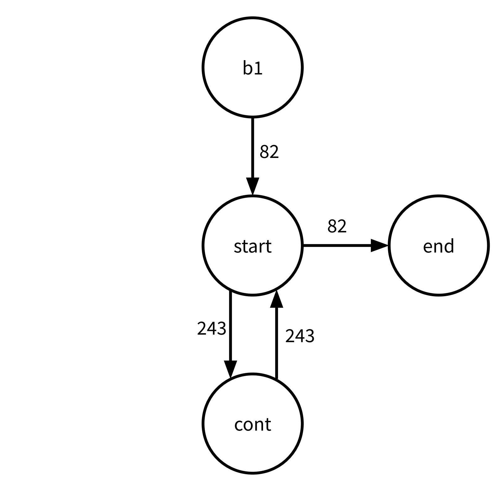
This is very similar to the weighted CFG for main. The output block order is the same: b1, start, cont, and end.

Putting all this together, the optimized Bril program is below (after running both function reordering and block reordering).

main {
  zero: int = const 0;
  one: int = const 1;
  val: int = const 1;
start:
  exp_zero: bool = eq exp zero;
  br exp_zero end cont;
cont:
  val: int = call multiply val base;
  exp: int = sub exp one;
  jmp start;
end:
  print val;
  ret ;
}
multiply {
  zero: int = const 0;
  one: int = const 1;
  curr: int = id zero;
start:
  b_zero: bool = eq b zero;
  br b_zero end cont;
cont:
  curr: int = add curr a;
  b: int = sub b one;
  jmp start;
end:
  ret curr;
}

When testing, I found the above program to have 29% fewer instruction pointer jumps than the unoptimized program when run on the same workload. We will now explore the evaluation of these optimizations.

Evaluation

I evaluated these optimizations by comparing the total number of instruction pointer jumps for the unoptimized and optimized programs on a given workload. I wrote six Bril programs and ran each with three workloads. On average, across all programs and workloads, function reordering decreased the total number of instruction pointer jumps by 7.7% with a standard deviation of 36%. Basic block reordering decreased the number of instruction pointer jumps by approximately 19%, with a standard deviation of 12%. Since the two optimizations do not interfere with each other, I also evaluated the combination of function reordering and basic block reordering, and found an average instruction pointer jump decrease of 12%, with a standard deviation of 35%. The high standard deviation of function reordering indicates that its performance is quite inconsistent and that the reordering algorithm has some serious flaws. I discuss this near the end of this section.

To conduct a thorough and rigorous evaluation of these optimizations, I ran them on numerous benchmark programs with various workloads. My evaluation strategy for a specific program was the following:

Profile the original program with a sample workload.
Run the function reordering optimization and profile with the same workload.
Repeat step 2 but with basic block reordering.
Repeat step 2 but run both optimizations one after another. Note that since the optimizations do not interfere, the order in which we apply the optimizations does not matter.
Repeat for all workloads.

I considered testing the optimized programs with a different "testing" workload but decided that this would not fairly evaluate the optimizations. Since we make the assumption that sample workloads are representative of real-world workloads, we should stick to that assumption.

Below is a graph showing the results of function and block reordering for 6 representative programs on three different workloads. Due to the lack of existing Bril programs to benchmark, I wrote the programs and their workloads. Each bar represents the corresponding program's average normalized number of instruction pointer jumps for the workloads, and the error bars represent the standard error. To normalize the instruction pointer jumps, I divided by the unoptimized program's number of instruction pointer jumps. This makes it easier to compare results for different workloads, as larger workloads will naturally have more total instruction pointer jumps. The last two programs do not contain any functions. Programs and workloads can be found here.

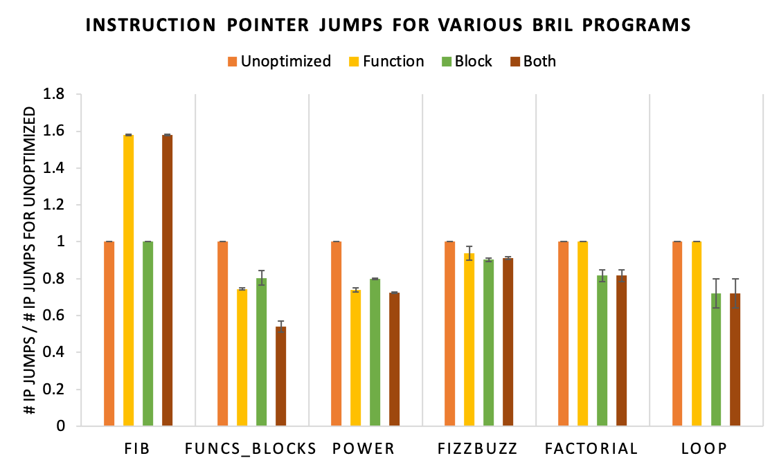
Note that the error bars for most programs are very small. The "Loop" test had quite large error bars, and this is because one of the workloads only ran one iteration of the loop, and this led to branching behavior to be quite different from the other workloads. For this workload, block reordering only gave a 0.6% increase in performance. This is important to note because it shows how the performance of the code layout optimizations is sensitive to the workloads.

From the above, we can see that the basic block reordering optimization consistently decreases the number of instruction pointer jumps by 10-20% (with the exception of the first test, which could not benefit from branch reordering), but the function reordering optimization is inconsistent. For "Fib", the function reordering optimization increased the number of instruction pointer jumps by approximately 59% on average. Below is the "Fib" benchmark.

main (n:int) {
  v1: int = call fib n;
  print v1;
}
le_one (n: int): bool {
  one: int = const 1;
  lto: bool = le n one;
  ret lto;
}
fib n: int {
  base: bool = call le_one n;
  br base return continue;
return:
  ret n;
continue:
  one: int = const 1;
  prev: int = sub n one;
  prev2: int = sub prev one;
  fib1: int = call fib prev;
  fib2: int = call fib prev2;
  ans: int = add fib1 fib2;
  ret ans;
}

And below is the optimized program returned by the function reordering algorithm.

main (n:int) {
  v1: int = call fib n;
  print v1;
}
fib n: int {
  base: bool = call le_one n;
  br base return continue;
return:
  ret n;
continue:
  one: int = const 1;
  prev: int = sub n one;
  prev2: int = sub prev one;
  fib1: int = call fib prev;
  fib2: int = call fib prev2;
  ans: int = add fib1 fib2;
  ret ans;
}
le_one (n: int): bool {
  one: int = const 1;
  lto: bool = le n one;
  ret lto;
}

Intuitively, this reordering makes sense. main calls fib, and fib calls le_one. However, note the location in fib where le_one is called. It is at the very top of the function—the first line in fact. As a result, when this call is made, the instruction pointer has to go down the entirety of fib to get to le_one, and then it has to go all the way back when le_one returns. In the original program, the instruction pointer only had to traverse the length of le_one, which is considerably shorter than fib. This demonstrates one of the core weaknesses of this function reordering algorithm. It assumes that all functions are of the same length and that on average, function calls are made halfway through a function. However, in real programs, this is rarely the case. I think it would be interesting to explore this further and see how we could incorporate the size of functions as well as the location of function calls to improve function ordering.

Conclusion

In conclusion, basic block reordering consistently decreased the total number of instruction pointer jumps, indicating that it improved code locality. On the other hand, function reordering did not always improve code locality, and in one case, increased the number of instruction pointer jumps by almost 60%. It would be interesting to investigate how function reordering could be improved to account for function lengths and function call locations. Ultimately, I found implementing these optimizations to be very interesting as they are quite different from classic optimizations.

The CS 6120 Course Blog