Probabril

by Oliver Richardson, Michael Roberts October 2, 2019

Introduction

Often one would like to represent a non-deterministic process as a combination of operations. Such a representation is often much more compact and often much more clearly represents the process you have in mind, and is easier to edit than conditional probability tables; a probabilistic program is one such way of representing such a program. All that was needed to do to turn bril into a probabilistic programming language is to add a source of randomness---in our simple case, a coin flip operation. Running such a program, gives you a sample from the distribution.

Of course, having the source code, we can do much more than running programs.

The Goal: An Exact Solver

The main bit of the project was to write an abstract interpreter that solves for the exact distribution that a probabilistic program represents. For instance, the program below flips two coins:

  x : bool = flip;
  y : bool = flip;
  ret

we should be able to see represents the distribution

$$ p \left(\begin{matrix} x \land y \\ x \land \lnot y \\ \lnot x \land y \\ \lnot x \land \lnot y \end{matrix}\right) = \left(\begin{matrix} .25 \\ .25 \\ .25 \\ .25 \end{matrix}\right)$$

By repeatedly running a program and recording the frequencies of resulting environments (Monte Carlo sampling), one can get a rough approximation of the distribution, but this can be less than satisfying for a number of reasons:

• The resulting distribution is only likely to be approximately correct
• This distribution will likely be very distorted in regions that are unlikely
• It can require exponentially many samples to resolve events
• Equally likely paths are likely to be close, but almost guaranteed not to have exactly the same mass estimate. Worse, no sampling method will ever be able to conclude that $p(x \land y) \not> p(x \land \lnot y)$ with high probability, regardless of the number of samples.

Instead, we can interpret the code as branching into two worlds on a flip, each tracking the exact correct amount of mass. While this works for straight line code, such as the program above, any loop which could run an unbounded number of times will cause the program to run forever. At this point, we have removed the probabilistic component, and we now have a deterministic approximation which will converge to the answer we would like. This alleviates the most pressing of our issues, but it is mildly annoying that we will never terminate when evaluating a program with possibly unbounded iteration, even if the limit point is obvious. For instance, this program which repeatedly flips two coins until one of them lands tails:

start:
  x : bool = flip;
  y : bool = flip;
  z : bool = and x y;
  br z start end;
end:
  ret

which one can easily see results in the distribution

$$ p \left(\begin{matrix}x \land y \land \lnot z \vphantom{\frac{1}{3}} \\ x \land \lnot y \land \lnot z \vphantom{\bigg|} \\ \lnot x \land y \land \lnot z \vphantom{\frac{1}{3}} \end{matrix}\right) = \left(\begin{matrix} ~\frac{1}{3}~ \\ ~\frac{1}{3}~\vphantom{\bigg|} \\ ~\frac{1}{3}~ \end{matrix}\right) $$ ... will never terminate if we just split worlds on flips, because there's there's always non-zero mass on some run which has not terminated, even though the pattern is clear, and the same computation has already been done in each iteration.

The goal is to design an algorithm which soundly deals with issues like this, which exactly computes distributions over any program with finite state space in a finite number of steps.

What I Did

I built an abstract interpreter which exactly (to reiterate: neither approximately, nor probabilistically) solves for the distribution of any program with finite state space, together with tools for generating random programs for evaluation, as well as some tools for observing and looping programs. To the best of my knowledge, everything like this that already exists is an iterative approximation of the fixed point, rather than exact calculation of the limit point. However, the procedure is simple enough that I would not be at all surprised if it had been done.

Despite the fact that we conceptually have done something cool, the distinction between exact and approximate may ultimately be in irrelevant, for a couple of reasons:

• In difficult cases of interest, distributions are continuous, and so this technique does not work.
• The approximations quickly converge to arbitrary precision, and so if you know what tolerance you want, it is sufficient to just run a few more iterations.
• As we will see the standard approach for probabilists does involve solving exactly, but only once you have calculated the eigenspace; it is easy to overlook the fact that computing eigenvectors / values is already an approximate algorithm, as standard libraries do this for you quickly at machine precision.

Other notable exact solvers include the PSI Solver, 2016, which handles continuous distributions, but requires straight line code (it unrolls loops), and Holtzen et. al.,'s Symbolic Exact Inference for Discrete Probabilistic Programs, 2019 which uses a much more efficient representation than ours, but also operates on programs with no control flow. The solvers that operate on arbitrary control structures, such as this one, all seem to be approximate (but again, converge to the true distribution up to machine precision quickly).

Design

To the language specification I have added three instructions,

• flip: an instruction which stores a random boolean in its target destination
• obv: an "observe" primitive, used for conditioning, which can be thought of as an assert---if it fails, the world and any mass on it are destroyed, netting a sub-distribution. If one thinks of programs as being normalized distributions (that is, conditioned on a program finishing), then this mass is re-distributed to the other runs, and this instruction is equivalent to a restart of the program.
• clear: clears the environment variables, removing all bindings.¹ obv can be compiled to a branch which restarts the program, with a clear.

Background on Exact Inference of Posterior Distribution

There are at least two canonical ways of approaching this problem: one from programming languages, and one from ergodic theory. In both cases, a program $P$ can be thought of as a weighted graph $(\mathcal S, T)$, where the vertices $$ \mathcal S := \mathrm{Instructions} \times \mathrm{Env} $$

are pairs consisting of the program counter and the environment state, and the weight $T_{s_1, s_2}$ of the edge between states $s_1$ and $s_2$ is the probability of transitioning from state $s_2$ from state $s_1$. Note that this graph is incredibly sparse, as each state can only move to one or two other states.

[ 1 ] Abstract Interpretation and Jacobi Iterates

The first thing we can do is in the same spirit as data flow analysis: we interpret programs abstractly---that is, run them by keeping track of some restricted information that necessarily must be true about each variable, rather than its exact value.

Consider the abstract domain $\mathcal D = ({\Delta \mathcal S}, \preceq, s, \oplus)$ of sets of distributions over states, which we will call $\Delta \mathcal S$. $\mathcal D$ can be endowed with a natural order $\preceq$ on which $T$ is monotonic, making it a complete partial order (CPO), i.e., an ordered set with arbitrary suprema. Because it is a CPO and $f$ is monotonic, there is a least fixed point of $x$ of $f$ such that $x \succeq s$ for any $s \in \mathcal S$, computed by

$$ x := \mathrm {lfp}^{\preceq} (f,s) = \lim_{n \to \infty} f^{n} (s) $$

The values obtained by stopping at any given point are called the Jacobi iterates, and are the basis of Cousot style abstract interpretation. However, even if the state space $\mathcal S$ is finite, the set of distributions over them is decidedly not---and this procedure will not terminate. In practice, to get termination people sacrifice completeness to get a sound, terminating abstract interpreter, pulling tricks such as widening. In this setting, this corresponds to giving up on the exact probability distribution, and instead reporting an upper probability.

The distribution of interest is the restriction of this fixedpoint $x$ to the program points that are return values, renormalized if thought of as a distribution rather than a sub-distribution.

[ 2 ] Stationary Distributions on Markov Chains

The second common view of a probabilistic program is as a Markov chain. In a very clear way, a program describes exactly the data required to transition from one state (including both the environment variables and the program counter) to a distribution over next states. In particular, the transition $\mathbf T_{i,j}$ is the probability of transitioning to state $j$ given that you're in state $i$. For a deterministic program, for instance, $\mathbf T_{i,j}$ is a function, and therefore has exactly a single one in each row, and zeros elsewhere. A fixed point here is a stationary distribution for the matrix $\mathbf T$---that is, an eigenvector associated to eigenvalue 1.

Projecion into Eigenspaces

Given an oracle for computing the eigenvectors of this transition matrix $\mathbf T$, the right thing to do is clear:

$$ \lim_{n \to \infty} \mathbf T^n \vec s = \lim_{n \to \infty} \mathbf U \Sigma^n \mathbf V^T \vec s $$

where $\mathbf U \Sigma \mathbf V^T$ is the singular decomposition of $\mathbf T$---that is, $\mathbf U$ and $\mathbf V$ are unitary and $\Sigma$ is a diagonal matrix of the singular values of $\mathbf T$. Because we know $\mathbf T$ is a (sub)stochastic matrix, we know that it can have no eigenvalue greater than 1, and if the program has any chance of returning, the return statement corresponds to an eigenvector that does in fact have corresponding eigenvalue 1. It is easy to see that any singular value that is less than 1 will ultimately go to zero, and so really we are just projecting the start state $\vec s$ into the eigenspace associated to the eigenvalue 1. If there are $k$ dimension of this eigenspace, we can write the previous equation as

$$\lim_{n \to \infty} \mathbf T^n \vec s = \mathbf U_k \mathbf V_k^T \vec s$$

where $\mathbf U_k$ and $\mathbf V_k$ are the first $k$ left and right eigenvectors of $\mathbf T$, respectively. This process is widely considered the standard solution to problems like ours.

However, there are a number of drawbacks of just implementing the algorithm like this:

1. It requires having fully explored the graph
2. Calculations of SVD and eigendecomposition do not benefit much from sparsity.
3. We already know most of the eigenvectors associated to eigenvalue 1: the ret statements. (The others correspond to infinite loops.)
4. Eigenvectors / eigenvalues must themselves be computed iteratively rather than exactly, due to the Abel-Ruffini theorem: in general, a matrix could have an arbitrary characteristic polynomial, and solving for eignenvalues means giving roots of this polynomial---and therefore eigenvalues cannot be calculated with algebraic operations in general so long as $| \mathcal S | > 5$.

Algorithm

The key insight is that the limit point of a single cycle can be computed the moment you spot the cycle, and know where all of the "off-ramps" are. For instance, if your program looks like this:

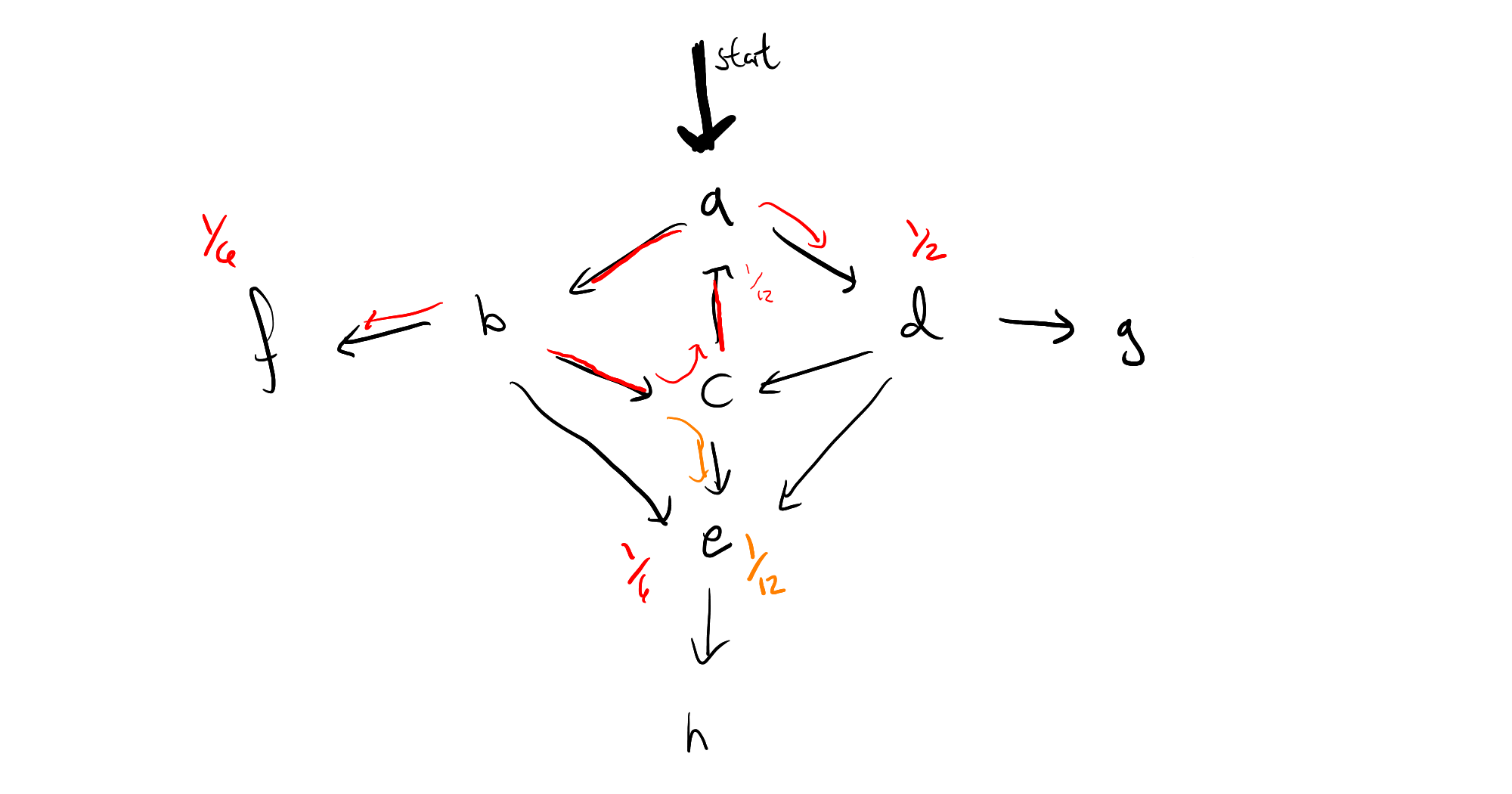
then the moment you've seen the path $a \to b \to c$, and realized that the probability mass has dropped from $1$ to $\frac{1}{8}$ by going around the circle, we see that that we will ultiately end up with a geometric series

$$ 1 + \frac{1}{12} + \frac{1}{12^2} + \frac{1}{12^3} + \cdots = \frac{1}{1 - \frac{1}{12}} $$

That is, we can immediately pass to a limit, by removing all weight at the origin of the cycle, and multiplying the probability masses which branch off by $\frac{12}{11}$, which means the resulting graph looks like this:

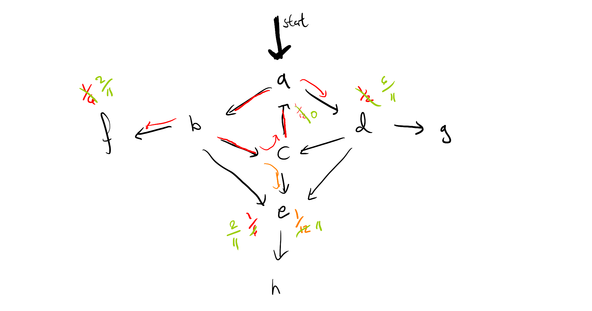
If we repeat this process for the left cycle in the graph, we'll see that we suddenly have mass back on node $a$ again, and so it may look as though all of this work hasn't really helped us after all, if we have multiple interacting cycles. This too can be overcome, by saving our work, in the form of a distribution frontier for each node, so that we can circumvent any duplicate calculations. I can use this intuition to give a rough sketch of a proof that algorithm will terminate (again, only for finite state space), but I have not yet investigated whether we can guarantee polynomial time.

In any case, here is the algorithm:

• Let $\texttt{best} : \text{Map}\langle \mathcal S, \Delta \mathcal S \rangle$ be initially a default dict with $(i,\text{env}) \mapsto \text{execInst}_i(\text{env})$.
• Initialize a queue $Q := []$.
• Repeat while $|Q| > 0$:
  • Dequeue $p := (i, \text{env}) \leftarrow Q$ from $Q$.
  • set $\texttt{best}[p] := \Big[\texttt{best}[p] / \texttt{best}[\textit{support}(\texttt{best}[p])]\Big]$; that is, extend the frontier of the distribution associated to $p$ by one level (or equivalently, use the monad multiplication $\mu$ to collapse $\texttt{best} \circ \texttt{best}$ to a distribution).
  • if $\text{weight}_p(\texttt{best}[p]) > 0$, i.e., if there is a cycle in $\texttt{best}[p]$:
    • $\texttt{best}[p] \leftarrow \texttt{best}[p] * \dfrac{1}{1 - \text{weight}_p(\texttt{best}[p])}$
    • $\text{weight}(\texttt{best}[p]) := 0$
  • append $\textit{support}(\texttt{best}[p])$ to $Q$; if this is non-empty, also append $p$.

What this looks like in terms of Power Iteration

If $\mathbf T = \Big[ t_{i,j} \Big]$, then we are only updating one line at once, and changing $\mathbf T$ at each iteration. To start off, we have a collection of matrices that look like this, for each $i$, which we plan on applying sequentially to $\vec s$:

$$ \begin{bmatrix}1 & & \cdots & & 0 \\ & 1 &&& \\ \Big[\text{---} & \text{---} & t_{i,j} & \text{---} & \text{---}\Big] \\ &&&1 & \\ 0 & & \cdots && 1 \end{bmatrix} $$

At each iteration, we combine adjacent ones together into a larger matrix via substitution / matrix multiplication, and save the result as the new vector $[- ~t_{i,j}~- ]$. Every time there is a cycle, i.e., positive mass in $t_{i,i}$ for some $i$, we pass immediately to the limit by redistributing the weight in $t_{i,i}$ to each of the other $t_{i,j}$ in proportion to their existing mass.

How is this possible given Abel-Ruffini?

While probabilistic Bril programs are not deterministic, they are far from being arbitrary matrices---because they're probabilistic transition matrices $A$ must have $\sum_{i} A_{i,j} = 1$ for all $j \in \mathcal S$. Moreover, because we already know the eigenvalues and even most of the eigenvectors we care about, there is no need to do some of this computation.

Implementation

This algorithm has been implemented in a file called xbrili, next to the normal interpreter brili. The code is available here.

The refactoring required to get this working include the following setup:

• Create a StringifyingMap whose keys can be other maps, so that we can index into our many maps and queues by program point.
• Expand Actions to also include splitting of worlds, for coin flips, and interpret instructions accordingly
• Push print statements in a buffer so they only complete at the end and once per run---unobserved runs won't print.

One can then roughly translate the pseudo-code above. There is no exploration before the algorithm starts; we directly traverse the instructions themselves, and build the $\texttt{best}$ map behind us as we go, just like any graph search algorithm. When we encounter back edges, we skip all of the interim computation and go directly to the frontier of the new node.

Extensions

There are several additional features of note in the implemented version beyond what has already been discussed. First, the more major elided details and extensions:

• I have also implemented an extension of this algorithm which backs off of finite space assumptions, by specifying a tolerance $t$. When the mass of a state $u$ from the state $s$ drops off enough, $\Pr(u \mid \vec{s}) < t$, we stop keeping track of the run entirely. It was actually rather hard to get this part right, because the algorithm relies on the queue both to track what still needs doing, and also to determine if a point changed after updating. There are many tempting resolutions involving just the queue, but all of the ones I tried came with subtle bugs. To fix this, I needed to separately track which program points had already finished, independent of the queue.
• I have also implemented a utility called random-bril.py which generates random Bril programs, with a mechanism for making sure that the distribution of different kinds of instructions is fairly even. There are a lot of parameters, so they are hard-coded. The parameters have been tuned to make things that look like reasonable programs to me, but of course do not reflect any real distribution of instructions, and there may be programs which are impossible to generate with it. Also, due to jumps, it is possible to generate programs that refer to variables before they are defined. We throw out any programs that generate errors like this.

And also some more minor or more technical details that may be of interest:

• brili now interprets flip as random, obv as a restart, and xbrili introduces new actions for world splitting.
• Printing is now delayed until the end of the execution and saved in the buffer, so that observations truly can totally undo everything and allow for a restart.
• There are options for removing the printing instructions entirely, and dumping environment variables at the end, for both interpreters, so that we can automatically test the correctness of the two against one another via random-bril.
• I have also added quite a bit to util.ts, including a way of indexing TypeScript Maps by other TypeScript Maps by means of stringification.

Difficulties

This took me a long time, and I was trying to figure out whether the algorithm I had in mind was sound, and how to get it to terminate, particularly once I didn't want to assume that my state space as finite right at the beginning.

Shortcomings in Algorithm

• In some cases I'm paying an extra factor of two: if there is a loop with an odd number of instructions, I have to go through the loop twice before the $\textt{best}$ map stabilizes. It is not clear there's an easy way of avoiding this, but it feels like there should be. Of course, "2 if you're unlucky" is much better than "as many as it takes to converge".
• The algorithm keeps revisiting nodes that it cannot possibly be done with yet. Rather than a queue, which gives this algorithm, or a stack, which looks more like a Gibbs Sampler, really the ideal is to have a priority queue, ordered by probability mass (where ties are broken by last time to arrival).
• I have sketch of a proof of soundness, but have not worked out the details. I also have not proved any complexity results.
• For a program with infinite state space, the algorithm might not terminate. Of course, this is unavoidable; the more pressing concern is that xbrili will use additional memory even if the original program runs in fixed space, which makes it much worse than executing a deterministic program. This could be alleviated by only saving things on branches; the trade off is that we lose opportunities to recognize the state we're in.
• A large number of the runs have the same control flow; these take up a lot of extra storage space.
• The algorithm we use here, to follow coin flips, does not transfer to continuous variables whatsoever. Resolving this is the subject of the second project.

Shortcomings in Implementation

• In backing off of the finite state space assumption, I have given only one mechanism for throwing out traces: if they have mass less than some tolerance. Other, arguably more useful criteria include, a global total tolerance,
• The priority queue idea was not implemented mostly because it seemed like a premature optimization, and the data structure we use to index it is mutable, so it would have been an additional engineering burden.

Evaluation

Example Programs

There are more examples in /test/prob/, for those interested. We will highlight two important ones:

Thirds

Consider the program we wrote earlier:

main {
start :
  x: bool = flip;
  y: bool = flip;
  z: bool = and x y;
  br z start end;
end:
  ret;
}

This outputs our desired thirds distribution, immediately and exactly:

[ 'done', Map { 'x' => true, 'y' => false, 'z' => false } ] 0.3333333333333333
[ 'done', Map { 'x' => false, 'y' => true, 'z' => false } ] 0.3333333333333333
[ 'done', Map { 'x' => false, 'y' => false, 'z' => false } ] 0.3333333333333333

We can also consider the de-looped version of this, where we use an obv instruction instead of a branch, explicitly killing mass and representing a sub-distribution:

main {
  a3: bool = flip;
  a2: bool = flip;
  print a3 a2;

  a1: bool = or a3 a2;
  obv a1;
  print a1;
}

this results in the following output:

[ 'done', Map { 'a3' => true, 'a2' => true, 'a1' => true } ] 0.25
[ 'done', Map { 'a3' => true, 'a2' => false, 'a1' => true } ] 0.25
[ 'done', Map { 'a3' => false, 'a2' => true, 'a1' => true } ] 0.25

which can easily be re-normalized to $\frac{1}{3}$ in each case if necessary, but reflects the fact that some of the mass was killed rather than looped. The difference will become important if we integrate probabril with functions---the exact place that you restart to, and when you renormalize, make a big difference, and if there are many places one could return to, there may be multiple natural choices.

Backing Off of Finite State Space

The following program, which has a counter, could have an unbounded number of states.

main {
  one : int = const 1;
  y : int = const 0;
reflip:
  x : bool = flip;
  y : int = add y one;
  br x reflip end;
end:
  ret;
}

Below is its output (with the constant field removed so that it fits more cleanly on the screen). Note that we have again solved for the exact distribution for every run that has a probability of more than $10^{-7}$, and also where the remaining program mass is after pushing the program this far.

[ 2, Map { 'y' => 24n, 'x' => true } ] 5.960464477539063e-8
[ 6, Map { 'y' => 24n, 'x' => false } ] 5.960464477539063e-8
[ 'done', Map { 'y' => 23n, 'x' => false } ] 1.1920928955078125e-7
[ 'done', Map { 'y' => 22n, 'x' => false } ] 2.384185791015625e-7
[ 'done', Map { 'y' => 21n, 'x' => false } ] 4.76837158203125e-7
[ 'done', Map { 'y' => 20n, 'x' => false } ] 9.5367431640625e-7
[ 'done', Map { 'y' => 19n, 'x' => false } ] 0.0000019073486328125
[ 'done', Map { 'y' => 18n, 'x' => false } ] 0.000003814697265625
[ 'done', Map { 'y' => 17n, 'x' => false } ] 0.00000762939453125
[ 'done', Map { 'y' => 16n, 'x' => false } ] 0.0000152587890625
[ 'done', Map { 'y' => 15n, 'x' => false } ] 0.000030517578125
[ 'done', Map { 'y' => 14n, 'x' => false } ] 0.00006103515625
[ 'done', Map { 'y' => 13n, 'x' => false } ] 0.0001220703125
[ 'done', Map { 'y' => 12n, 'x' => false } ] 0.000244140625
[ 'done', Map { 'y' => 11n, 'x' => false } ] 0.00048828125
[ 'done', Map { 'y' => 10n, 'x' => false } ] 0.0009765625
[ 'done', Map { 'y' => 9n, 'x' => false } ] 0.001953125
[ 'done', Map { 'y' => 8n, 'x' => false } ] 0.00390625
[ 'done', Map { 'y' => 7n, 'x' => false } ] 0.0078125
[ 'done', Map { 'y' => 6n, 'x' => false } ] 0.015625
[ 'done', Map { 'y' => 5n, 'x' => false } ] 0.03125
[ 'done', Map { 'y' => 4n, 'x' => false } ] 0.0625
[ 'done', Map { 'y' => 3n, 'x' => false } ] 0.125
[ 'done', Map { 'y' => 2n, 'x' => false } ] 0.25
[ 'done', Map { 'y' => 1n, 'x' => false } ] 0.5

Even though there is still some symmetry left to be desired (a more satisfying solution could be given by widening perhaps), note that assembling a picture like this via Monte Carlo would take an insane number of samples. Effectively we have done power iteration, but for a space which we did not know was finite beforehand.

Random Testing

Due to the number of parameters and computing time required to make the random testing reasonable, this bit of the evaluation is less conclusive than I was hoping it would be. Nonetheless, the infrastructure is all there. probabril/random-tester.py generates a program, xbrili, and then many instances of brili --noprint --envdump, doing a $\chi^2$ test on the resulting output frequencies of environment variables.

Here is a sample output of 10 random programs, with 100 samples. The first number is the $\chi^2$ statistic, then the $p$-value, and then the expected and observed frequencies.

chi2 0.36 p 0.5485 	 (50, 50) (47, 53)
chi2 4.0 p 0.26146 	 (25, 25, 25, 25) (20, 20, 30, 30)
chi2 0.0 p nan 	 (100,) (100,)
chi2 1.20 p 0.7530	 (25, 25, 25, 25) (23, 26, 22, 29)
chi2 3.52 p 0.3181 	 (25, 25, 25, 25) (21, 23, 23, 33)
chi2 0.64 p 0.4237 	 (50, 50) (54, 46)
chi2 0.24 p 0.970 	 (25, 25, 25, 25) (23, 26, 26, 25)
chi2 0.64 p 0.423 	 (50, 50) (46, 54)
chi2 4.88 p 0.180 	 (25, 25, 25, 25) (19, 34, 23, 24)
chi2 18.6 p 0.0092 	 (12, 12, 12, 12, 12, 12, 12, 12) (4, 14, 19, 8, 9, 13, 12, 21)
chi2 1.96 p 0.1615 	 (50, 50) (57, 43)
chi2 2.72 p 0.2564 	 (50, 24, 24) (53, 29, 18)


random programs that could not be executed by xbrili due to undefined variables: 3

Low $p$-values are bad, because they suggest that the expected distribution is different from the observed one. However, when this happens there are a few explanations for this---not only are the sample sizes very low, but also I had to set a very aggressive timeout for the interpreter to avoid the numerous infinite loops, which results in a count of zero for some programs which may have terminated.

Nonetheless, one can see that the expected frequencies mirror the expected ones. One might worry that this sample does not include many interesting programs with control flow that generates things with more than powers of two---and this is largely true, but every once in a while it does happen, and anecdotally xbrili still gets them right.