Induction Variable Optimizations
Induction Variables
Loops are well known targets for optimization since they execute repeatedly and significant execution time is spent in loop bodies. The class of loop optimizations which we're considering in this post are centered on special variables called induction variables (IVs). An induction variable is any variable whose value can be represented as a function of: loop invariants; the number of loop iterations that have executed; and other induction variables.
Generally speaking, most induction variable optimizations are limited to
induction variables that are linear functions of their inputs.
For Bril, that means induction variables are computed only using
the mul, add and ptradd instructions.
Optimization Overview
There are a large number of induction variable optimizations which all have slightly different goals. Here, we're going to give a brief overview on some of the optimizations we implemented and what they're meant to achieve.
Strength Reduction
In reality (despite what many software developers like to think), not all instructions are really created equal. Some instructions are more expensive to execute at runtime than others. For instance, integer addition is usually "cheaper" than integer multiplication. Induction variable strength reduction lets us "reduce" multiplication operations on IVs to addition operations.
Take this simple program as an example:
int j = 0;
for (int i = 0; i < 100; i++) {
    j = 2*i;
}
return j;
j is an induction variable dervied by applying a multiplication
to another IV, i. This makes it a perfect candidate for strength
reduction. Each iteration we set j to a brand new value
computed with that multiplication. Instead, every iteration we can increment j
by two times whatever we increment i by.
To simplify this optimization this is usually done by introducing a new variable
to represent the 2*i value for each iteration.
int j = 0;
int s = 0; //2*i when i == 0
for (int i = 0; i < 100; i++) {
  j = s;
  s = s + 2; //+2 since i gets incremented by 1 each iteration
}
After some other common compiler optimizations, we can get this simpler version:
int j = 0;
for (int i = 0; i < 100; i++) {
  j = j + 2;
}
return j;
It's important to note that j no longer has a direct dependence on i
since there are no instructions which read from i and write to j.
Strength reduction often helps remove data dependencies, paving
the way for other IV optimizations.
Induction Variable Elimination
In many programs, IVs can be redundant.
For instance, a common programming idiom is to introduce
a variable only to use as a loop guard (such as i in the following program).
int max = 10;
int result = 0;
for (int i = 0; i < max; i++) {
    result += 2;
}
return result;
In this example, we can eliminate the i variable
by replacing its uses with another basic induction variable result to get:
int max = 10;
int result = 0;
for (; result < max*2; result+=2) {}
return result;
This obviously removes extraneous code by combining the "loop counting" part of the loop with the actual work that it's doing.
Implementing Induction Variable Optimizations
It turns out that IV analyses require a large number of other static analyses before even thinking about optimization.
Finding Loops
For instance, IV optimizations are all loop optimizations, which means we need to identify loops. Natural loops are denoted by sets of basic blocks that all have a common entry point and a "backedge" in the control flow graph. This backedge corresponds to a branch or jump in the CFG that goes back to the beginning of the loop. Finding loops requires finding backedges, which it turns out requires calculating dominators. A backedge is defined as any edge in the control flow graph where the source vertex is dominated by the sink. Therefore to even start thinking about optimizing we need to calculate the dominators and do a basic reachability analysis. See the pictures below for an example CFG with backedge annoations.
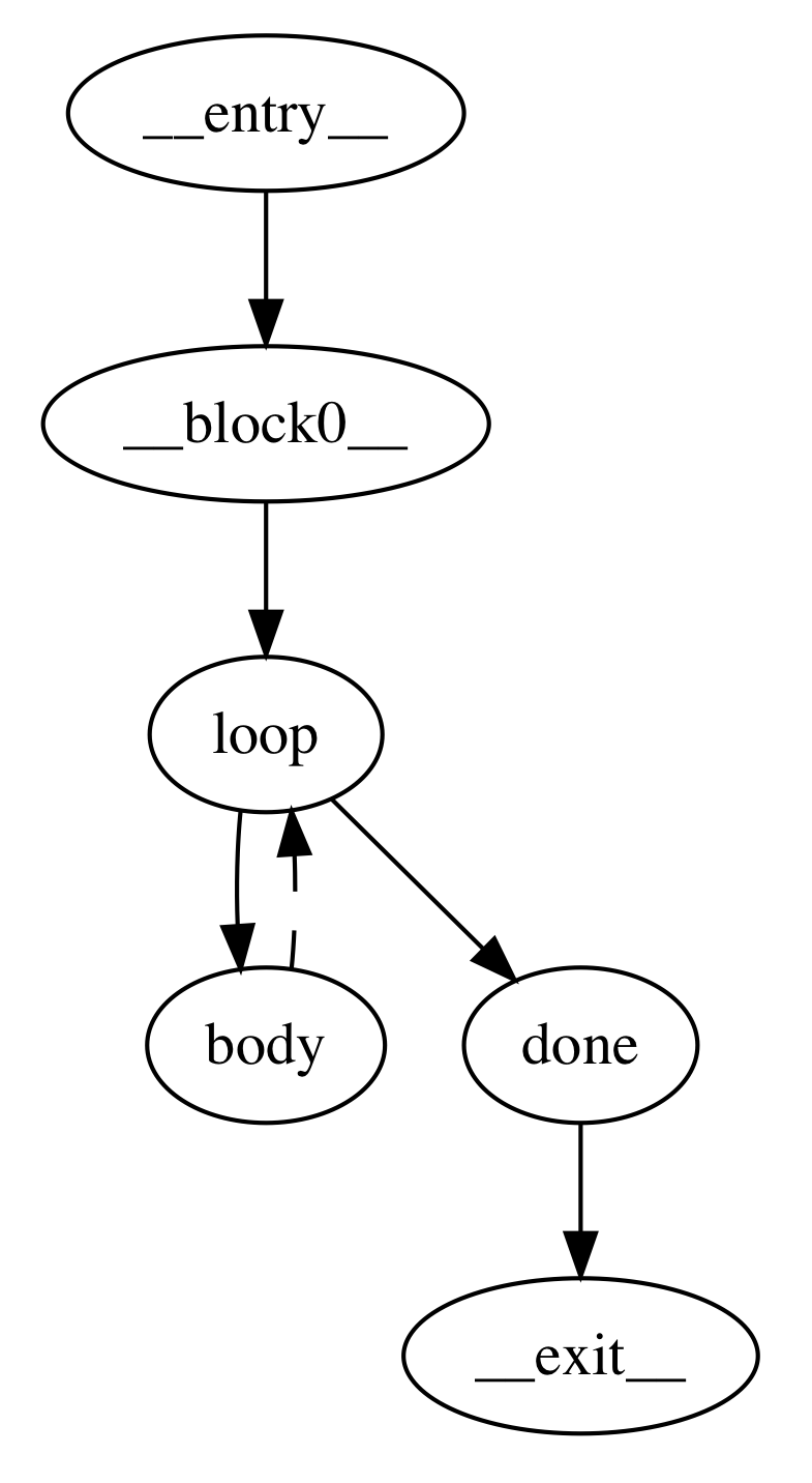
 On the left hand side we have the control flow graph where its only backedge
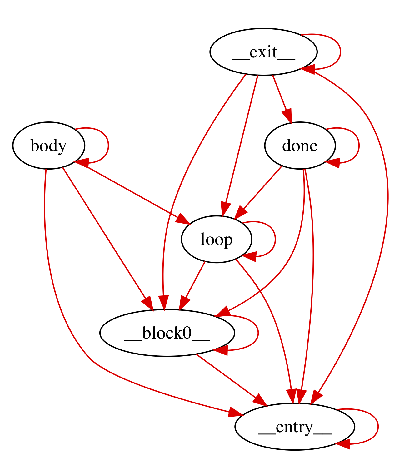
is represented as a dashed line. The right hand side picture shows all of the
dominators; each red line can be read as "is dominated by." As you can see,
the only edge in the CFG which is the reverse of an edge in the dominator graph
is the backedge from
On the left hand side we have the control flow graph where its only backedge
is represented as a dashed line. The right hand side picture shows all of the
dominators; each red line can be read as "is dominated by." As you can see,
the only edge in the CFG which is the reverse of an edge in the dominator graph
is the backedge from body to loop.
There are some other subtleties here with nested loops or two loops which happen to have the same entry block. In these cases, we combine these overlapping loops into a single loop. Otherwise we could incorrectly identify or re-write IVs by looking at incomplete information. This approximation of loop structure prevents our analysis from finding some optimization opportunities but preserves correctness.
Identifying Induction Variables
Once we find loops, then we need to figure out which variables exactly are
induction variables. We divide IVs into two categories: basic induction variables;
and derived induction variables. The most common examples of IVs are the
loop variables that are only used for loop tests (say i in the following code):
for (int i = 0; i < 100; i++) {
  A[i] = 0;
}
However, basic IVs are more generally defined:
A basic induction variable, X, is a variable whose only updates within the loop are of the form X = X + c, where c is loop-invariant.
In Bril, c is always a variable (as opposed to an inlined constant) so we need to do some sort
of analysis to determine if instruction operands are loop-invariant.
We use a reaching definition
analysis to find such variables. We consider any variable to be loop-invariant
if: 1) all of its definitions which reach the loop entrance originate outside
the loop; or 2) it has only one reaching definition which is a const expression.
In our implementation we only identify a subset of basic IVs, specifically those that are updated precisely once inside the loop. We did this for simplicity, since it greatly reduces the complexity of future IV optimizations. An elegant way to deal with this complexity would be to run IV optimizations on SSA code, since all variables have only one definition.
In addition to basic IVs, derived IVs are also eligible for optimization. A derived IV is:
A variable with exactly one definition inside the loop whose value is a linear function of loop-invariants and a basic IV.
There are several methods for finding derived IVs, the most general one being a dataflow analysis. We decided to implement a simpler but probably less efficient and less complete approach that just involved scanning all of the definitions in the loop and collecting a set of definitions which satisfy the above constraints.
In Bril, in particular, our algorithm can be
very approximate. Since each definition can only implement
one operation, there may be derived IVs which are comprised of multiple
Bril defintions. For example, in Bril, x = 3*i + 4 looks like:
x:int = mul i three; //three has been defined as const 3
x:int = add x four;  //four has been defined as const 4
Our code doesn't consider x an induction variable because
of our very approximate heuristic: "x is updated twice in the
loop, so it may not be an IV."
Induction Variable Representation
In most compilers, induction variables have a standard representation,
which we also adopt. Every induction variable is symboliclly stored
as a tuple of the form (i, a, b) where i is a base IV.
You can read this as induction variable x = ai + b; a neat consequence
of this representation is that base induction variables are all of the form (i, 1, 0)
since i = i*1 + 0. In our compiler, a and b can be the name of any loop-invariant variable.
This representation is easy to serialize into a sequence of Bril instructions.
Liveness
Since induction variable elmination is meant to delete unnecessary variable assigments, we need to be truly sure that those induction variables are not used outside of the loop's scope (or ensure that we update its final output value at the end of the loop). We use a liveness dataflow analysis to compute all of the "live-ins" and "live-outs" of every basic block.
Unfortunately, this isn't enough for eliminating "useless" induction variables. Consider the following Bril-esque C program:
int max = 10;
int result = 0;
int i = 0;
LOOP:
  if (result < max*2) //live-ins = [result, i, max]
    goto BODY;
  else
    goto END; //live-outs = [result, i]
BODY:
  result = result + 2; //live-ins = [result, i]
  i = i + 1;
  goto LOOP; //live-outs = [result, i]
END: // live-ins = [result]
return result;
Even though i is used only to update itself,
a standard liveness analysis says that i must be both a live-out and a live-in
for all of the loop blocks. This prevents local dead code analyses from removing the useless update: i = i + 1.
Instead of local liveness, we need to consider the live-outs of the entire loop.
Therefore, when considering the liveness of IVs that we're trying to eliminate,
we don't check the live-outs of any one basic block.
Instead, we union all of the live-ins of the
loop's successors. If i is not in that set of variables, we know that no code
which executes after the loop will use i and we can safely delete it.
In the example above, the only successor to the loop is the END block
and therefore the only live-out of the loop is result.
Strength Reduction Implementation
Strength reduction targets derived IVs, specifically. Our implementation attempts to apply this optimization to all derived IVs in the program. Since strength reduction can increase the total dynamic instruction count (in some cases) and code size (in all cases) you might imagine using some heuristic to decide when to apply this optimization.
Otherwise, our implementation is very standard and follows this
algorithm to optimize derived IV x = (i, a, b):
- Before the beginning of the loop, create a fresh variable
fand initialize it tof = a*i + b - Replace the one assignment to
xin the loop withx = f - Immediately following the update to
i, insert the updatef = f + a
Our implementation is somewhat naive and inserts a number of id
and other instructions which can be eliminated by copy propagation.
Step (3) from the above algorithm is simplified since we ensure that
basic induction variables are updated only once in the loop. If we were to
allow multiple updates to i we'd need to follow the correct update to i.
Basic Induction Variable Elimination
After running strength reduction, we attempted to eliminate all basic induction variables from the program. We chose to run this following strength reduction since that optimization often removes dependencies on basic IVs. The first step of IVE is to chose a derived IV to replace the basic IV. This was another opportunity for applying heuristics to guide our optimizations; instead, we chose which derived IV to use arbitrarily. Once we picked this IV, we iterated over all comparisons in the loop which used the basic IV as an argument and a loop-invariant variable as the other argument. For each of these comparisons we replaced the basic IV with the derived IV and inserted instructions to compute the appropriate value of the other argument. Since the other argument was loop-invariant, we lifted these instructions outside of the loop (this is very similar to step (1) of strength reduction).
For example, in this C code, if k is an IV of the form (i,3,5) and n is loop-invariant:
if (i < n) {
  ...
}
We can replace i and n in this conditional with the following:
if (k < 3*n + 5) {
  ...
}
This transformation removes uses of i and can likely eliminate all uses except for the use in the write to itself (i = i + c). If this is the case, and i is not a live-out of the loop we can remove this assignment (as mentioned before, global DCE won't normally remove this update). Our implementation does delete such dead code.
Note that, even if i is a live-out, it's sometimes possible to push this i = i + c update to the end of the loop so that it is not part of the loop body; however, we didn't implement this due to its complexity and questionable utility.
At this point we have successfully removed all traces of i from the loop. i might still be used to initialize some of the strength reduction variables in the beginning of the loop. However, if i is initialized to a constant, this can probably be eliminated with constant propagation and simple dead code elimination.
Evaluating Our Optimizations
In order to evaluate our optimization, we modified the brili Bril interpreter to also optionally output the breakdown of dynamically executed instructions by opcode. This allowed us to quantify both the effect on total dynamic instruction count and validate the impact of strength reduction. Nevertheless, these results are not indicative of real world performance gains. In particular, while being interpreted, it is unlikely that strength reduction will yield a significant (if any) real time speedup. Furthermore, if the Bril that we generate was compiled using something like LLVM, different processors may have different costs for adds and multiplies, which may render strength reduction less useful. Nevertheless, these measurements are a good indication that our pass is doing what it is supposed to (reducing the number of typically expensive operations).
In order to get some measurements for our optimization, we created a test suite of several different types of programs. One type of program is a "sanity check" program, which is a small program on which we could predict how our optimizations would perform. These helped us validate the correctness of our optimizations. The other type of program is a "real world" program, which is supposed to represent a real world task in order to see what kind of performance improvements we can get on more realistic programs. Of the programs below only fib and mat_mul_8 are what we would consider "real world" programs (although they are of course still small examples).
The following table breaks down dynamic instructions counts for each of the programs we tested:
| Program | Loop Iterations | Total ICBase | Total IC Opt | mul Count Base | mul Count Opt | add Count Base | add Count Opt | ptradd Count Base | ptradd Cont Opt | id Count Base | id Count Opt |
|---|---|---|---|---|---|---|---|---|---|---|---|
| array | 8 | 95 | 118 | 0 | 2 | 24 | 24 | 16 | 18 | 2 | 18 |
| array_mul | 8 | 113 | 136 | 17 | 5 | 24 | 40 | 16 | 16 | 2 | 18 |
| strength | 30 | 187 | 193 | 30 | 3 | 60 | 60 | 0 | 0 | 0 | 30 |
| strength_large | 1000 | 6007 | 6013 | 1000 | 3 | 2000 | 2000 | 0 | 0 | 0 | 1000 |
| fib | 48 | 642 | 700 | 0 | 4 | 194 | 98 | 146 | 150 | 0 | 144 |
| mat_mul_8 | 512 | 10828 | 11076 | 2048 | 541 | 2632 | 2704 | 1728 | 1728 | 3 | 1539 |
Test Descriptions:
- array: Accesses several arrays with an index variable for each array.
- array_mul: The same as array but the acceses use multiplication to calculate array offsets.
- strength: A simple loop that should be a good candidate for strength reduction.
- strength_large: Strength but executing more loop iterations.
- fib: Calculates the first 50 fibonacci numbers and stores them into an array.
- mat_mul_8: Multiplies two 8x8 matricies. Note that this test starts with 588 matrix initialization instructions which are common to all executions (none of the initializers are multiplies).
Evaluation Conclusions
We conclude from the above results that our strength reduction optimization is very successful at replacing multiplications with additions and additions with copy instructions; however on programs with few loop iterations, it's unclear whether or not this optimization will be "worth it." However, the generation of so many id instructions (and our analysis of the outputs of the toy programs) suggests that future optimization passes would be able to eliminate many of the ineffeciently-generated instructions here. After executing those passes, it is likely that total instruction count overhead would disappear.
The second half of our pass, which eliminated basic induction variables, we believe had little impact. Unfortunately, our implementation was structured such that it is difficult to test one without the other; we only removed uses of a variable when we applied strength reduction to one of its derivatives. However, this is easy to intuit and our manual inspection of the code confirms this. Removing the update to a single basic IV corresponds to removing # of loop iteration instructions. While this is at least an improvement that scales with execution time, it is still minor.
Evaluation Weaknesses
Our evaluation (and implementation) have a few salient weaknesses. First, we should have evaluated against all of our test programs on a number of different inputs. We neglected to do this primarily because of time and the triviality of the results. Obviously removing instructions from the inner loop bodies would reduce the occurrences of costly instructions more as the number of loop iterations increases. To demonstrate, we included the strength_large example in our suite. In this case, the additional overhead (even without copy prop or dce) was only 7 instructions but vastly reduced the number of multiplications.
Originally we sought out to implement general induction variable elimination optimizations; unfortunately strength reduction ended up being our primary success. For instance, a canonical use case for IVE is transforming:
int[] A,B;
for (int i=i1=i2=0; i < max; i++) {
 A[i1++] = B[i2++];
}
Into:
int[] A,B;
for(int i=0; i < max; i++) {
 A[i] = B[i];
}
Our implementation will not successfully execute this optimization (this case is essentially the array test from our test suite).
In this example i, i1 and i2 are all basic induction variables. Our implementation relies on replacing one basic IV with a derived IV
from its family. In this example, the optimization requires replacing one basic IV with another. We would have liked to implement this optimization given more time since it covers the most common case for induction variable elimination. Lacking this feature explains why we saw some useful optimization in the array_mul test but nothing in the array test.
Correctness
We also added a set of correctness tests to verify that running our induction variable optimizations did not break anything. We paid particular attention to including programs with multiple loops that had interesting control structure. For example, we included programs that had loops with branches and multiple backedges corresponding to the same loop entry point. All of our correctness regression tests pass, so our optimizations are (hopefully) sound.