Software Simulation for Data Streaming in HeteroCL
With the pursuit of higher performance under physical constraints, there has been an increasing deployment of special-purpose hardware accelerators such as FPGAs. The traditional approach to program such devices is by using hardware description languages (HDLs). However, with the rising complexity of the applications, we need a higher level of abstraction for productive programming. C-based high-level synthesis (HLS) is thus proposed and adopted by many industries such as Xilinx and Intel. Nonetheless, to achieve high performance, users usually need to modify the algorithms of applications to incorporate different types of hardware optimization, which makes the programs less productive and maintainable. To solve the challenge, recent work such as HeteroCL proposes the idea of decoupling the algorithm from the hardware customization techniques, which allows users to explore the design space and the trade-offs efficiently. In this project, we focus on extending HeteroCL with data streaming support by providing functional software-level simulation (in contrast with hardware-level simulation, where we simulate after hardware synthesis). Experimental results show that with LLVM JIT runtime, we can have orders of speedup compared with the software simulation provided by HLS tools.
Why Data Streaming?
Unlike traditional devices such as CPUs and GPUs, FPGAs do not have a pre-defined memory hierarchy (e.g., caches and register files). Namely, to achieve better performance, the users are required to design their memory hierarchy, including data access methods such as streaming. In this project, we focus on the streaming between on-chip modules. The reason that we are interested in the cross-module streaming is that it introduces more parallelism to the designs. To be more specific, we can use streaming to implement task-level parallelism. We use the following example written in HeteroCL to illustrate the idea of streaming.
@hcl.def_([A.shape, B.shape, C.shape])
def M1(A, B, C):
    with hcl.for_(0, 10) as i:
        B[i] = A[i] + 1
        C[i] = A[i] - 1

@hcl.def_([B.shape, D.shape])
def M2(B, D):
    with hcl.for_(0, 10) as i:
        D[i] = B[i] + 1

@hcl.def_([C.shape, E.shape])
def M3(C, E):
    with hcl.for_(0, 10) as i:
        E[i] = C[i] - 1

M1(A, B, C)
M2(B, D)
M3(C, E)
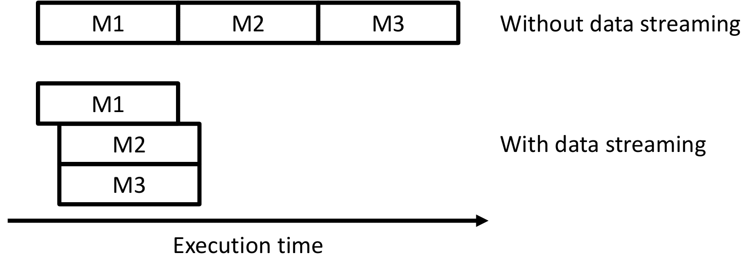
In this example, M1 takes in one input tensor A and writes to two output tensors B and C. Then, M2 and M3 read from B and C and write to D and E, respectively. We can see that M2 and M3 have no data dependence and can thus be run in parallel. Moreover, these two modules can start as soon as they receive an output produced by M1. To realize such task-level parallelism, we can replace the intermediate results B and C with data streams. We illustrate the difference between before and after applying data streaming with the following figure.
Data Streaming in HeteroCL
The key feature of HeteroCL is to decouple the algorithm specification from the hardware optimization techniques, which is also applicable to streaming optimization. To specify streaming between modules, we use the primitive to(tensor, dst, src, depth=1). It takes four arguments. The first one is the tensor that will be replaced with a stream. The second one is the destination module and the third one is the source module. Finally, users can also specify the depth of the stream. Currently, the data stream is implemented with FIFOs. HeteroCL will provide other types of streaming in the future. Following, we show how to specify data streaming with our previous example.
s = hcl.create_schedule([A, B, C, D, E])
s.to(B, s[M2], s[M1], depth=1)
s.to(C, s[M3], s[M1], depth=1)
Software Simulation for Data Streaming
It is not enough with the programming language support only. We also need the ability to simulate the programs after applying data streaming. One way to do that is by using the existing HeteroCL back ends. Namely, we can generate HLS code with data streaming and use the HLS tools to run software simulation. Note that the software simulation here refers to cycle-inaccurate simulation. The reason why we only focus on cycle-inaccurate simulation is that to complete cycle-accurate simulation, we need to run through high-level synthesis, which could be time-consuming in some cases. We can see that the existing back ends require users to have HLS tools installed, which is not ideal for an open-source programming framework. Moreover, the users will need a separate compilation to run the simulation. Thus, in this project, we introduce a CPU simulation flow to HeteroCL by extending the LLVM JIT runtime. With this feature, users can quickly verify the correctness of a program after adding data streaming.
Implementation Details
The code can be seen here. The key idea is to simulate data streaming with threads. In other words, each module will be executed using a single thread. We also implement a scheduling algorithm to decide the firing of a thread and the synchronization between threads. For streaming, we implement the streams by using one-dimensional buffers. We assign the size of a buffer according to the specified FIFO depth. Currently, we only provide blocking reads and blocking writes. Non-blocking operations will be left as our future work. In the following sections, we describe the algorithms and implementation details.
Module Scheduling
The purpose of this algorithm is to schedule each module by assigning it with a timestep, which indicates the execution order between modules. Namely, modules that can be executed in parallel are assigned with the same timestep. Similarly, if two modules are executed in sequence, they are assigned with different timesteps. Note that the numbers assigned to two consecutive executions do not need to be continuous. Since each module is executed with a single thread, a thread synchronization is enforced between two consecutive timesteps.
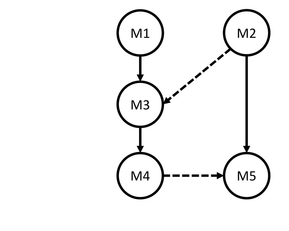
To begin with, we first assign each module with a group number. Modules within the same group are executed in sequence, while modules in different groups can be executed in parallel. To assign the group number, we first build a dataflow graph (DFG) according to the input program. An example is shown in the following figure, where the solid lines mean normal read/write operations while the dotted lines refer to the read/write of data streams.
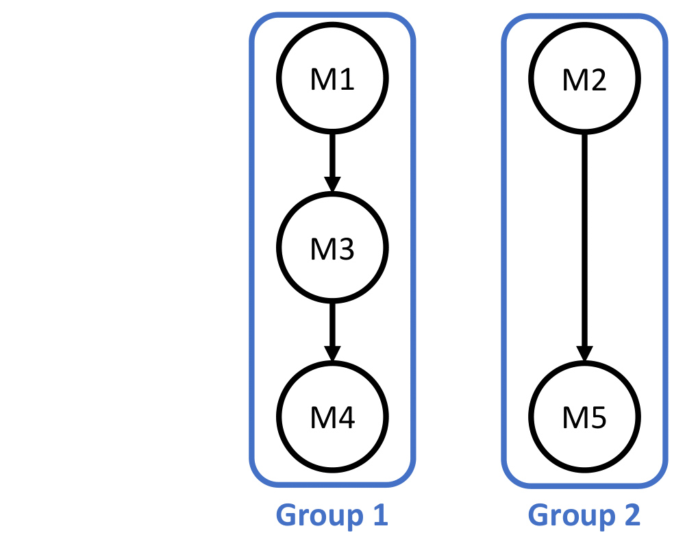
After the DFG is built, we remove all the dotted lines. Then, we assign a unique ID to each connected component. This ID will be the group number. An example is shown below.
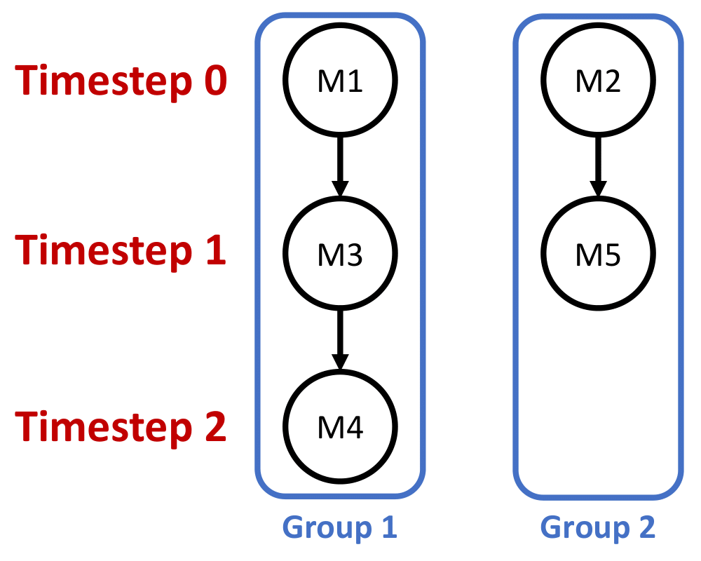
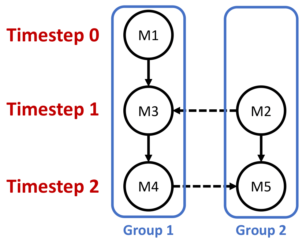
Now, we can start the scheduling process by assigning the timestep to each module. We first perform a very simple as-soon-as-possible (ASAP) algorithm. Namely, the first module within each group will be assigned with timestep 0. After that, we assign the timestep of each module according to the data dependence. An example is shown below.
However, this is not correct because as we mentioned above, modules connected with streams should be run in parallel. Namely, they will share the same timestep. To solve that, we add one dotted line back at a time and correct the timesteps. We also need to correct its succeeding modules accordingly. After all dotted lines are added, we finish our scheduling algorithm.
Note that there exist cases where we cannot solve. For example, if two modules A and B are connected with a solid line, and the producer A streams to a module M while B also streams from M, then there exists no valid scheduling according to our constraints. One possible way to solve that is by merging A and B into a new module A_B. In this case, the streaming from/to M becomes an internal stream, which can be scheduled easily by assigning A_B and C with the same timestep. The reason why in this implementation we do not merge the two modules is that it is possible that we reuse A or B for other computations. In this case, we will need to reconstruct the DFG. Thus, we leave this as our future work.
Parallel Execution with Threads
After we assign each module with a timestep, we can start to execute them via threads. Before we execute a module with a new thread, we check whether all modules assigned with smaller timesteps are completed. In other words, we first check whether all modules assigned with smaller timesteps are fired. If not, we schedule the current module to be executed in the future by pushing it into a sorted execution list. Then, if all modules with smaller timesteps are fired, we check whether they are finished. If not, we perform thread synchronization (e.g., by using thread.join() in C++). Finally, we need to execute the modules in the execution list. Since the list is sorted, we do not need to worry about new modules being inserted into the list.
Stream Buffers
In this work, we implement the streams with buffers that act like FIFOs. Instead of popping from or pushing to the buffers, we maintain a head and a tail pointer for each buffer. The pointers are stored as integer numbers. The head pointer points to the next element that will be read from, and the tail pointer points to the next element that will be written to. We update the pointers each time an element is written to or read from the buffer. We need to perform modulo operations if the pointer value is greater than the buffer size (i.e., FIFO depth). Since we may have two threads updating the pointers at the same time, we use std::atomic provided by C++ to make sure there is no data race. Finally, we maintain a map so that we can access a stream according to its ID.
LLVM JIT Extension
To enable users with a one-pass compilation, we extend the existing LLVM JIT runtime in HeteroCL. It is complicated and hard to maintain if we implement both threads and stream buffers using pure LLVM. Thus, we implement them with C++ and design an interface composed of a set of functions. For instance, we have BlockingRead, BlockingWrite, ThreadLaunch, and ThreadSync. Then, inside our JIT compiler, we call the functions by using LLVM external calls.
Evaluation
In this section, we evaluate our implementation by using both unit tests and realistic benchmarks. Experiments are performed on a server with 2.20GHz Intel Xeon processor and 128 GB memory. We verify the correctness of the final result and compare the total run time in different cases.
Unit Tests
The tests can be found here. Following we breifly illustrate what each test does by using the DFGs.
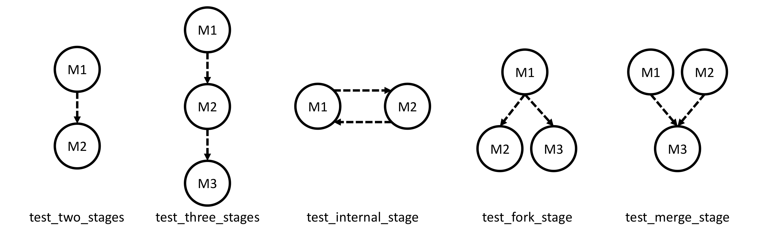
For unit tests, we compare the run time before and after applying data streaming. The results are shown in the following table. We run the results for 1000 times and calculate the average.
| Testcase | Original (ms) | Multi-threading (ms) | Speedup |
|---|---|---|---|
| two_stages | 0.0592 | 0.0554 | 1.070 |
| three_stages | 0.0831 | 0.0715 | 1.162 |
| internal_stage | N/A | 0.0638 | N/A |
| fork_stage | 0.0865 | 0.0758 | 1.141 |
| merge_stage | 0.0906 | 0.0739 | 1.226 |
The average speedup of our test cases is 1.150, which makes sense because now we use multi-thread execution. Note that for the third benchmark (i.e., test_internal_stage), the functionalities are different before and after applying data streaming. To be more specific, we list the test program here.
@hcl.def_([A.shape, B.shape, C.shape, D.shape])
def M1(A, B, C, D):
    with hcl.for_(0, 10) as i:
        B[i] = A[i] + 1
        D[i] = C[i] + 1

@hcl.def_([B.shape, C.shape])
def M2(B, C):
    with hcl.for_(0, 10) as i:
        C[i] = B[i] + 1

M1(A, B, C, D)
M2(B, C)

s = hcl.create_schedule([A, B, C, D])
s.to(B, s[M2], s[M1], depth=1)
s.to(C, s[M1], s[M2], depth=1)
We can see that without applying streaming, the production of D is not affected by M2. However, if we specify C to be streamed from M2 to M1, the original memory read of C in M1 now becomes a blocking read. This also demonstrates that without the simulation support for streaming, some hardware behaviors cannot be correctly represented.
Realistic Benchmark
We also show the evaluation results from a realistic benchmark, which is more complicated than the synthetic tests in the unit tests. Due to time limitation, we only use the Sobel edge detector, which is a popular edge detecting algorithm in image processing. We compare the results with the software simulation tool provided by the HLS compiler. More specifically, we first generate Vivado HLS code with hls::stream. Then we use csim to run the software simulation. The evaluation results are shown below. We also show the time overhead due to compilation.
| Simulation Method | Simulation Time (s) | Compilation Overhead (s) | Total Run Time (s) |
|---|---|---|---|
| LLVM JIT | 0.00094 | 0 | 0.00094 |
| Vivado HLS csim | 1.63 | 1.29 | 2.92 |
We can see that with LLVM JIT runtime, we can have orders of speedup compared with HLS simulation. Moreover, the overhead caused by compilation is not negligible for HLS simulation.
Conclusion and Future Work
In this work, we implement a software simulation runtime for data streams in HeteroCL by extending the existing LLVM JIT back end. We implement the simulation runtime with multi-threading in C++. Moreover, we propose a scheduling algorithm that exploits the task-level parallelism of a program after applying data streaming. Finally, we use unit tests to verify our work and use a realistic benchmark to demonstrate the programming efficiency over existing HLS tools.
Our next step will be testing our extension with more realistic benchmarks. In addition, by parsing HLS reports, we may be able to perform the cycle-accurate simulation. Then we can compare the performance of our scheduling algorithm with those implemented in existing HLS tools. In the end, we want to submit a pull request to the upstream HeteroCL repository.