Dynamic Edge Profiling with Optimal Counter Placement
Introduction
For this project, we wanted to implement an LLVM pass that dynamically profiled basic block edges. The naïve implementation would be to add a profiling mechanism to every edge in the program, but that comes with a significant amount of overhead. To minimize overhead, we strived to add profiling to the minimum number of edges necessary to obtain the same amount of profiling information. The key insight is that we can determine if an edge is traversed using profiling information from preceding and succeeding edges if the CFG structure ensures the program can only run through a simple path between those profiled edges.
Algorithm
To select the edges to profile, we used Knuth's algorithm:
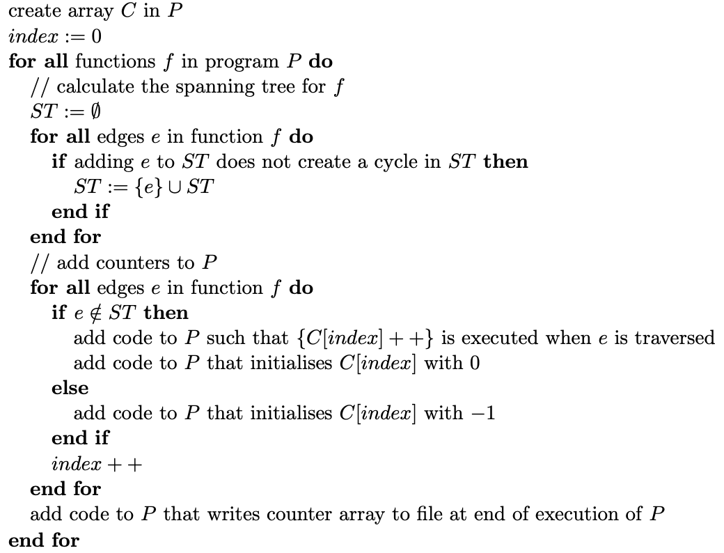 ---
Essentially, this algorithm first finds the minimum spanning tree of the edges in a function and then adds profiling instrumentation---code that logs profiling information---to all edges not in the spanning tree. Note that this algorithm uses the first block in a function as the root of the spanning tree, and that edges are treated as bidirectional when checking for cycles.
---
Essentially, this algorithm first finds the minimum spanning tree of the edges in a function and then adds profiling instrumentation---code that logs profiling information---to all edges not in the spanning tree. Note that this algorithm uses the first block in a function as the root of the spanning tree, and that edges are treated as bidirectional when checking for cycles.
This algorithm works because the acyclic nature of the spanning tree entails that there is exactly one path between any two instrumented edges (or the entry or exit of the function). Thus, logging the traversal of one instrumented edge implies traversal of the program through the path from the previously logged edge location to the current one. This also implies that this is the minimum number of instrumented edges because having one less instrumented edge would either create a path that could be traversed without logging any profiling information or create multiple paths that lack sufficient profiling information to deduce which path was taken.
Offline Edge Count Extrapolation Algorithm
After we run our program, we know the number of times our instrumented edges were traversed. In order to determine the number of times the remaining edges were produced, we need to do some post-processing of our CFG with our runtime results.
The idea behind this algorithm is to iterate over the edges and fill in the edge count until convergence. The program will converge under the assumption that the edge profiling information supplied is sufficient to determine the rest of the edge counts. It is valid to fill in an edge count if there is a simple path between two nodes with known edge count. You can find detailed pseudocode and proofs for this offline algorithm in this dissertation by Andreas Neustifter.
Implementation
We wanted our instrumentation implementation to be as noninvasive as possible for the base code as pervasive changes could make the LLVM IR harder to reason about and could prevent future optimizations. To achieve that, we implemented the bulk of the profiling information logging in a separate runtime library file. This strategy allows us to reduce instrumentation to two function calls, one to logsrc(num1) in the edge's "source" block and one to logdest(num2) in the "destination" block, both of which reside in the library file. These functions calls take in a block-unique integer (num1 and num2 above) that is generated during the pass as arguments, meaning that we can identify an edge traversal with a pair of logsrc(num1), logdest(num2) function calls. The unique integers were simply the order in which the blocks were iterated through in our pass.
This approach allows us to leave the CFG unchanged, which would not be the case if we took the straightforward approach of adding a new block in the "middle" of every edge to hold the profiling code.
Since the function arguments are unique for each block, this means at most one logsrc(num1) and logdest(num2) is necessary in each block. To log each edge traversal, the runtime library keeps track of the order in which those functions are called as it is possible to trigger one of those functions without having traversed an edge with profiling instrumentation, though this does not impact correctness as the functions would not be triggered as a logsrc-logdest pair (and thus would not cause profiling information to be logged). For example, a natural loop's backedge, from block A to block B (where B is the loop header) could be instrumented. In this case, A would contain a logsrc(num1) call and B would contain a logdest(num2) call. B's logdest(num2) call would be triggered whenever the program enters the loop header, but since that call was not immediately preceded by the matching logsrc(num1) from A, the runtime library will know that the A→B edge traversal did not actually happen so no profiling information is logged. In some rare cases, there may be a path from a block with logsrc(num1) to logdest(num2) that does not go along the instrumented edge (i.e., it takes another routhe through multiple un-insturmented blocks), so in those cases we add a function call to logdisrupt(num3) in the first node on the un-instrumented path to signal that an alternative route was taken.
As the profiling logic and data are written in a runtime library disjoint from the LLVM pass, this information can be outputted however the user wants with minor edits to the library file. We chose to print it to standard out for simplicity. There is also the matter of correlating the block numbers assigned during the LLVM pass to the actual blocks, and this is done by printing the block-to-number matching for the source and destination blocks of each instrumented edge to standard out during the pass.
Evaluation
Correctness
To measure performance, we ran a subset of C benchmarks from the LLVM test suite. We collected the tabulated results and CFGs to manually verify our instrumentation was on an optimal number of edges with correct edge counts. We ran the algorithm described above to extrapolate the uninstrumented edges. We include one test here for visibility. Consider the following CFGs for a program with two functions, main and testFunc.
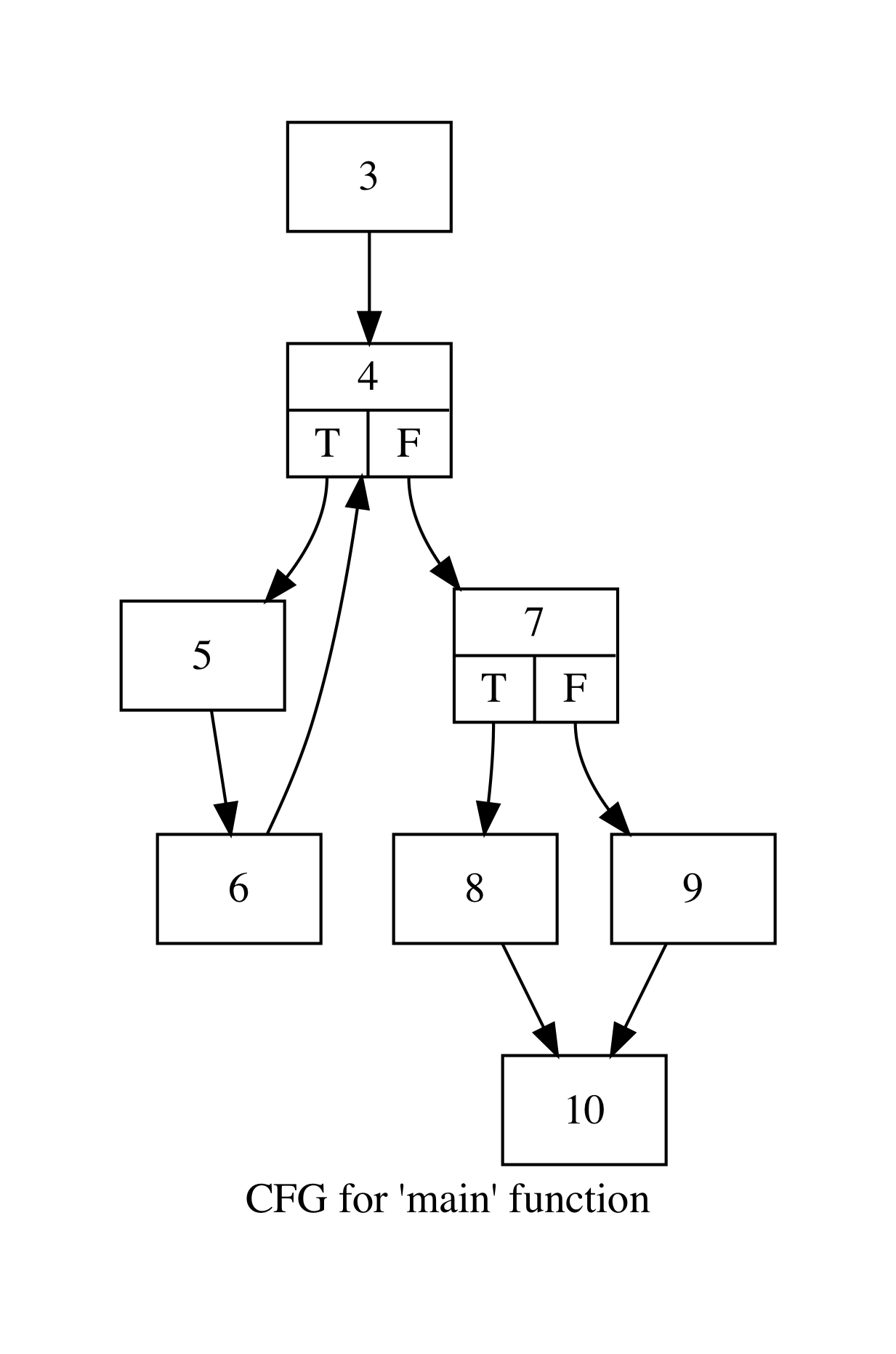
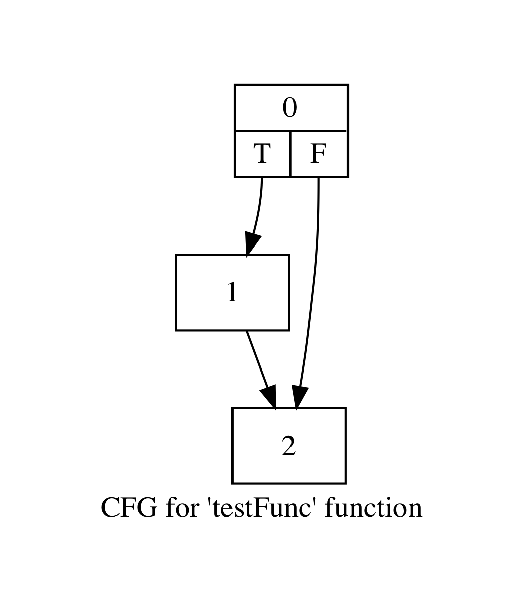 We run our instrumented program with input argument `5` and procure the table below.
| Edge | Count |
|---|---|
| [6->4] | 5 |
| [9->10] | 1 |
When we ran our pass, we also output the edges that were instrumented.
These edges were [0->2], [6->4], and [9->10].
To verify these results, we consider our program.
void testFunc(int n){
    if(n%2==1) printf("The number is odd\n");
}

int main(int num) {
    for(int i =0; i<5; i++){
        printf("Iteration %i\n", i);
    }
    if(num%2 == 0){
        printf("The number is even\n");
    }
    else{
        testFunc(num);
    }
    printf("%i\n", num + 2);
    return 0;
}
In order to automatically verify these results, we implement a naïve LLVM pass for edge profiling that instruments every edge. We then compare the results collected and extrapolated from optimal edge profiling with the results from running the naïve implementation.
Consider the results from running the naïve implementation.
| Edge | Count |
|---|---|
| [1->2] | 1 |
| [3->4] | 1 |
| [4->5] | 5 |
| [5->6] | 5 |
| [6->4] | 5 |
| [7->9] | 1 |
| [9->10] | 1 |
We confirm that our results for optimal placement match the results from naïve placement. In order to verify the remaining edges, we run the extrapolation algorithm discussed above by hand. The next step is to implement the extrapolation and automatically verify that the optimal placement pass produces the same results as the naïve pass for all edges.
We showed one test here, and performed similar analyses on several tests we designed with tricky CFGs in terms of loops and function calls.
To measure optimality in terms of the number of instrumented edges, we run the algorithm by hand on a few of our test CFGs. We find that our implementation results in the same number of instrumented edges as we expect. While we would like to automate this process, we were unable to find an LLVM pass that did similar edge count profiling to compare against.
Performance
We used C benchmarks from the LLVM test suite. Specifically, we used single-source benchmarks as we did not want support instrumenting external files/libraries and complex build processes. There were 66 total (we excluded a few that had unusual clang compilation or linking errors). For each program, we measured the performance after these three stages of passes:
- original code → LLVM
-O3 - original code → LLVM
-O3→ Our Profiling Pass - original code → LLVM
-O3→ Our Profiling Pass → LLVM-O3
We ran each stage 3 times per program.
On average, we found that adding profiling takes 5x longer than the unprofiled code, and the optimized profiling takes 4.8x longer than the unprofiled code.
Below are our performance results. The data has been normalized to the average runtime for each program's original code after LLVM -O3. This means that if a bar's height is 2, that stage's average runtime took 2x longer than the optimized but unprofiled code.
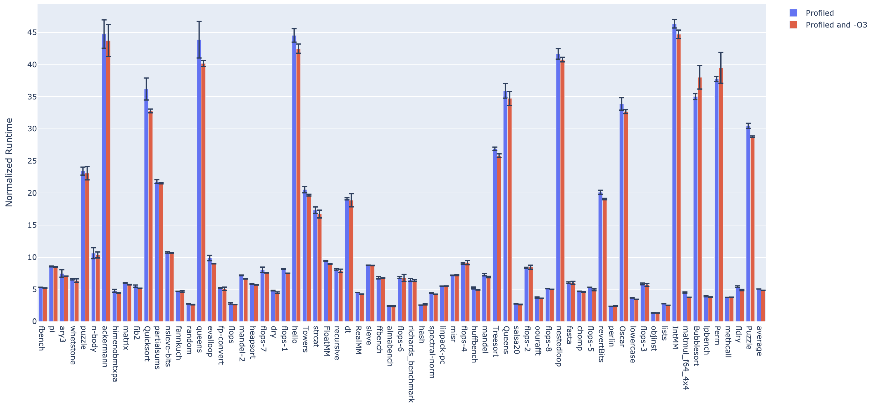
A next step to further improve performance would be to place counters on edges that are less likely to be executed, decreasing the number of dynamic instructions. This can be done by additional profiling and then creating a maximum spanning tree using the estimated edge weights instead of an arbitrary spanning tree.
Challenges
One of the primary challenges of this project was correctly installing LLVM on each of our machines with the correct version and /include/ directories. When planning our design, we utilized several online resources that varied quite a bit in terms of targeted LLVM version. Available source files change quite a bit, and therefore we realized we needed to be more aware of the version of LLVM these resources were using when reading them.
The other main challenge was figuring out how to work with LLVM. Part of this work encompassed determining the tools and information we had access to and what information we needed to collect manually. We found the most effective way to learn how to work with LLVM was from experimenting with examples. In particular, when implementing dynamic edge profiling, we found passes that implement other dynamic passes like dynamic instruction count to be especially helpful.
The source code for the LLVM pass detailed above can be found on GitHub.