CS612
(Homework 1)
0
Introduction
The file hw1.zip contains sources that you will need to complete the tasks of this assignment. There are three directories inside, one for each problem.
1
Problem
1: Detecting the Memory Hierarchy
In this problem you will empirically detect certain parameters of the memory hierarchy of a machine of your choice. Carefully examine the contents of the detect.cpp file inside the problem1 directory. When you feel confident that you know what the program does and how it does it, compile it with full optimization using your favorite compiler (we recommend g++, i.e. “g++ -O3 detect.cpp”) and run it on your favorite machine. The output consists of series of rows, following the general pattern:
<size> <stride>
<timing>
Plot the results on two different graphs (using Matlab, Excel, Gnuplot, or another plotting package):
- A 3D surface graph, with size and stride as base axes, using timing to generate the surface;
- A 2D line graph, which contains a separate line for each size, using stride for the X-axis and timing for the Y-axis.
Try putting timing on logarithmic scale. You will notice that in the provided data points size and stride, are already forming a logarithmic sequence. Here are two example graphs that you might get:
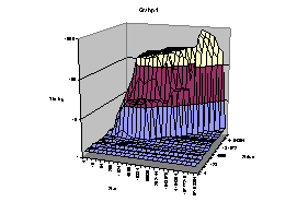
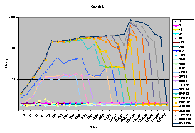
Examine closely the graphs and answer the following questions:
· How many levels of cache exist on the machine?
· For each cache level, find its capacity, line (block) size, associativity and miss penalty.
· Can you say anything about TLB and virtual memory, i.e. page size, number data TLB entries, …?
2
Problem
2: Miss Ratio as a Measure of Cache Effectiveness
One measurement of cache effectiveness (or accordingly how tuned one application is for the particular cache architecture) is the miss ratio, which is the fraction of memory references that miss in the cache. Obviously the lower the miss ratio, the more reuse gets exploited. In this problem we will measure the miss ratio for three common matrix algorithms and try to get some insight of using the results to perform high-level restructuring optimizations.
In order to compute the miss ratio, we are going to use a cache simulator. The simulator resides in the problem2 directory and currently simulates the ijk version of matrix-matrix multiply. Pay special attention to the file simulate.cpp. It contains the actual MMM simulation. Here is how it looks like:
#include
<iostream>
#include
<sstream>
using namespace std;
#include
"array2D.h"
#include
"array1D.h"
#include
"cachet.h"
#define S
(2 * 1024) // cache capacity
#define L
(32) // cache line size
#define A
(4) // cache associativity
#define E
(sizeof(double)) // matrix element
size
#define N
(100) // matrix size
void
main ()
{
Cache *cache = new CacheT<S, L, A>();
cache->Invalidate();
Array2D a(N, N, E, cache);
Array2D b(N, N, E, cache);
Array2D c(N, N, E, cache);
for (int i = 0; i < N; i++)
for
(int j = 0; j < N; j++)
for (int k = 0; k
< N; k++)
c(i, j, 3)
+= a(i, k, 1) * b(k, j, 2);
stringstream f;
f << N << "\t"
<< "ijk";
cout << cache->Statistics(f.str());
}
There are several notable differences from a real MMM. First you need to initialize the cache and invalidate it (empty it). Then declaring arrays (matrices) is now “Array2D <name>(<rows>, <cols>, sizeof(<type>), cache)” instead of just “<type> <name>[<rows>][<cols>]”. This permits the cache simulator to track array accesses in the following algorithm. One other difference is the array indexing: instead of just saying “<name>[<row>][<col>]” we use “<name>(<row>, <col>, <label>)”. The label argument is optional, but if specified, it allows the cache simulator to track the origin of all misses (i.e. tie a particular miss to a particular matrix). Finally we print the statistics gathered by the simulator, which in this case are:
100 ijk
1 0 0 1000000
100 ijk
1 4 0
250000
100 ijk
2 0 0
1000000
100 ijk
2 4 0
1000000
100 ijk
3 0 0
1000000
100 ijk
3 4 0
2500
100 ijk
3 0 1
1000000
100 ijk
1 1 0
2500
100 ijk
2 1 0
2500
100 ijk
3 1 0
2500
100 ijk
1 2 0
247500
100 ijk 2
2 0 997500
The first two columns were specified by us as a parameter to the Statistics function of the cache. Next column is the label (as specified as an additional parameter in the array references) – remember that we used 1 for A, 2 for B and 3 for C. If no label is specified in the references, expect to see only 0 here. Next column is the type of miss: 0=none, 1=cold, 2=capacity, 3=collision, 4=miss if the cache was fully associative. In summary, 0 in this column represents number of references; 1, 2, and 3 collectively represent the number of misses given the chosen cache organization; 4 represents the number of misses of a fully associative cache of the same size and same line size. Finally the next to last column represents the access type (0=read, 1=write) and the last column represents the count of references/misses.
The cache simulator simulates a write-allocate cache! Of course you can alternatively use a different cache simulator. We recommend using this one, as it is rather short, you have the whole implementation and it is quite fast as it does not generate memory reference traces, but does the simulation in real-time. When doing your experiments, plug-in the L1 data cache parameters that you found in Problem 1 for the cache capacity, line (block) size and associativity.
The simulator can be complied with Visual C++ or GCC (we have tried version 3.2). Remember to enable all optimizations as it makes use of some STL code, which is very slow if optimizations are not used:
g++ -O3 simulate.cpp
If you C++ library does not have a hash_map header, you might want to try –Dusemap parameter also.
Simulate the following programs for problem sizes 1 to N (where N is sufficiently large, to observer all the variations of the miss ratio) using some appropriate step, refining it in some regions to get detail where necessary:
· Matrix-Vector Multiply (MVM): 2 different loop orders: IJ and JI
· Matrix-Matrix Multiply (MMM): 6 different loop orders IJK, IKJ, JIK, JKI, KIJ, KJI
· Cholesky Factorization: 3 right-looking column versions (KIJ, KJI, KIJfused), 1 left-looking column version (JIK) and 1 row version (IJK):
do k = 1, N A(k,k) = sqrt (A(k,k)) do i = k+1, N A(i,k) = A(i,k) / A(k,k) do i = k+1, N do j = k+1, i A(i,j) -= A(i,k) * A(j,k) Code 1. KIJ right-looking column Cholesky Factorization |
do k = 1, N A(k,k) = sqrt (A(k,k)) do i = k+1, N A(i,k) = A(i,k) / A(k,k) do j = k+1, N do i = j, N A(i,j) -= A(i,k) * A(j,k) Code 2.KJI right-looking column Cholesky Factorization |
do k = 1, N A(k,k) = sqrt (A(k,k)) do i = k+1, N A(i,k) = A(i,k) / A(k,k) do j = k+1, i A(i,j) -= A(i,k) * A(j,k) Code 3. KIJ right-looking fused column Cholesky Factorization |
do j = 1, N do i = j, N do k = 1, j-1 A(i,j) -= A(i,k) * A(j,k) A(j,j) = sqrt (A(j,j)) do i = j+1, N A(i,j) = A(i,j) / A(j,j) Code 4. JIK left-looking column Cholesky Factorization |
do i = 1, N do j = 1, i do k = 1, j-1 A(i,j) -= A(i,k) * A(j,k) if (j < i) A(i,j) = A(i,j)/A(j,j) else A(i,i) = sqrt (A(i,i)) Code 5. IJK row Cholesky Factorization |
do {i,j,k} in 1 <= k <= j <= i <= N if (i == k && j == k) A(k,k) = sqrt (A(k,k)); if (i > k && j == k) A(i,k) = A(i,k) / A(k,k); if (i > k && j > k) A(i,j) -= A(i,k) * A(j,k); Code 6. General form of Cholesky Factorization with guards |
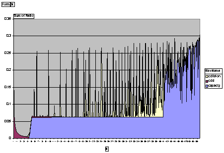
Explain the changes in the miss ratio on each graph (especially the sudden ones). Discuss the results and the opportunities they give us for performing high-level restructuring optimizations.
3
Problem
3: Miss Ratio as a Tile Size Predictor
Now you will investigate how to use miss ratio for predicting tile size. Based on your results from the previous problem, choose the best version (in your opinion) of MMM and then using its miss ratio graph choose an appropriate tile size to be used for tiling the three loops (using cubic tiles, i.e. equal in length in all dimensions).
You will try to verify the performance of your prediction by observing the miss ratio of tiled MMM. For that reason you need to measure the number of misses on all 36 versions of tiled MMM for different tile sizes… sounds like a long experiment, especially after your experience with waiting for the results of problem 2 to get out of the cache simulator. Therefore in this problem we will use the hardware counters in modern CPUs to count the number of misses.
In the problem3 directory you will find a library for programming and reading the hardware counters on the Intel P6 family of microprocessors (Pentium Pro, II, and III and selected Celeron versions) under the Windows operating system. You are free to search the net and use other libraries, possibly for different CPUs or OSes. If you have Pentium 4 and want to use it with this library, you still can, but it has a different micro-architecture and performance counters are accessed differently. Essentially you need to write a wrapper similar to P6Counter for P4. It is not a required part of this assignment and it is definitely not for the faint of heart. For this problem, the path of least resistance is to use a Windows machine with a P6 processor.
If you choose to use the library provided, please read the documentation in problem3\doc\install.htm and problem3\doc\index.htm to understand how to install and use the library respectively. You need to use Visual C++ this time. Take a look at problem3\p6demo\p6demo.cpp:
#include "ia32.h"
#include "p6counter.h"
void
main ()
{
p6counter
c1(p6counter::L2_REQUEST, p6counter::L2_MESI);
p6counter
c2(p6counter::DCU_MEMORY_REFERENCE);
const int c =
10000000;
static int a[c];
for (int ai1 = 0; ai1
< c; ai1++)
a[ai1]++;
SetPriorityClass(GetCurrentProcess(),
REALTIME_PRIORITY_CLASS);
uint64 t1 = c1;
uint64 t2 = c2;
for (int ai2 = 0; ai2
< c; ai2++)
a[ai2]
*= 13;
printf("L1
misses = %I64d\nL1 accesses =
%I64d\n", c1 - t1, c2 - t2);
}
This program counts the number of L1 data misses and memory accesses during a element wise multiplication by 13 of a big array of integers.
Measure the number of misses and references for the 36 version of MMM in a similar way for enough data points and plot the 36 lines on a graph with the problem size for X-axis and the miss ratio for Y-axis. Explain the results of the experiment. Were you right about the prediction? If not, how far was your prediction from the optimum?