Project 5 Part B: Diffusion Models
Implement and deploy diffusion models for image generation. The second part of a larger project.
Key Information
| Assigned | Thursday, April 17, 2025 (fork the starter code from Part A: GitHub Classroom, and Part B: GitHub Classroom) |
| Due |
Part A: Friday, April 25, 2025 (early due date): submit to
your Part A GitHub repo and CMSX by 8:00 PM Part B: Tuesday, May 6, 2025 (Extended): submit to your Part B GitHub repo and CMSX by 11:59 PM |
| Code Submission |
For each part, submit the following to your GitHub Classroom repository:
- Completed notebook file ( .ipynb) with figures and results- Python backup file ( .py) with your final implementation
Also save your Colab notebook with figures and results as a PDF and upload it to the corresponding CMSX assignment for Part A and Part B. |
| Individual Project | This project must be completed individually (no group work). |
Detailed Instructions for Part B
Overview
In Part B, you will train your own diffusion model on the MNIST dataset. This part focuses on understanding the training process of diffusion models, implementing the network architecture, and analyzing how well your model learns to generate data.
All work should be completed in the provided Colab notebook, available from GitHub Classroom.
Submission Instructions
Please submit the following to your Part B GitHub Classroom repository:
- The completed notebook file (
.ipynb) with your figures, results, and explanations - A Python backup file (
.py) with your final implementation
In addition, save your Colab notebook as a PDF and upload it to the CMSX assignment for Part B.
Tip: Start early! This part involves training a diffusion model, which may take time to run on Colab.
Part 1: Training a Single-Step Denoising UNet
Let's warmup by building a simple one-step denoiser. Given a noisy image
1.1 Implementing the UNet
In this project, we implement the denoiser as a UNet. It consists of a few downsampling and upsampling blocks with skip connections.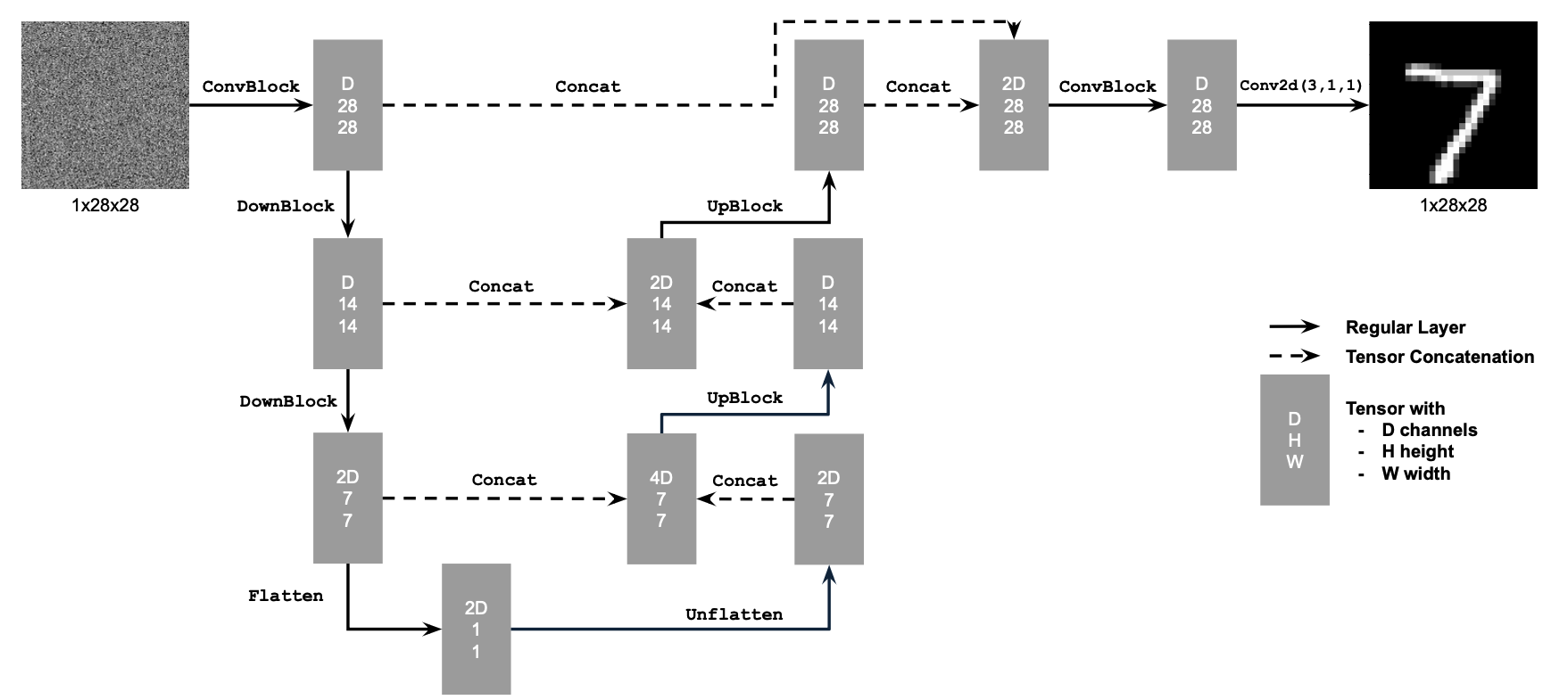
Figure 1: Unconditional UNet
The diagram above uses a number of standard tensor operations defined as follows:
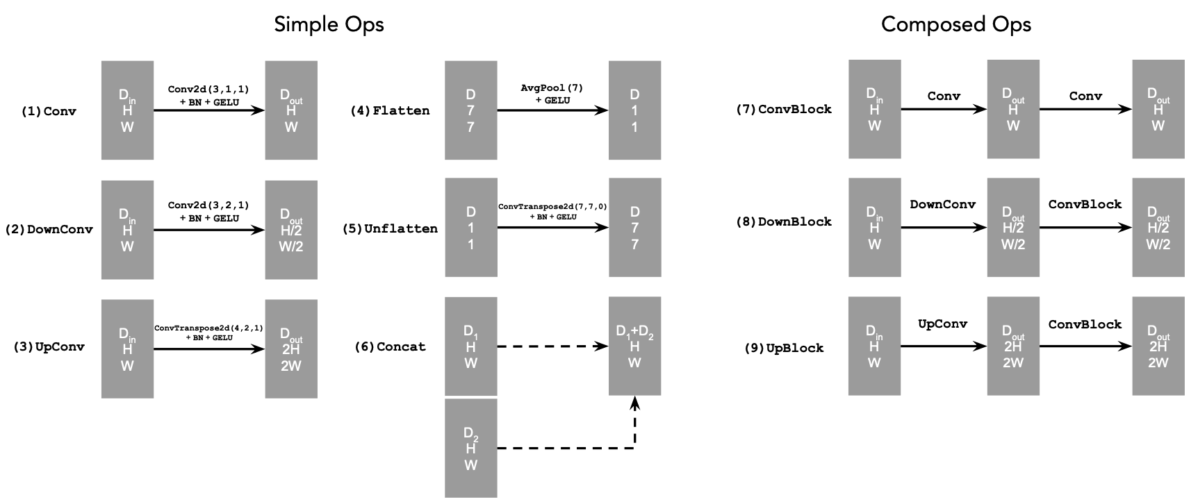
Figure 2: Standard UNet Operations
- Conv2d(kernel_size, stride, padding) is
nn.Conv2d() - BN is
nn.BatchNorm2d() - GELU is
nn.GELU() - ConvTranspose2d(kernel_size, stride, padding) is
nn.ConvTranspose2d() - AvgPool(kernel_size) is
nn.AvgPool2d() Dis the number of hidden channels and is a hyperparameter that we will set ourselves.
- (1) Conv is a convolutional layer that doesn't change the image resolution, only the channel dimension.
- (2) DownConv is a convolutional layer that downsamples the tensor by 2.
- (3) UpConv is a convolutional layer that upsamples the tensor by 2.
- (4) Flatten is an average pooling layer that flattens a 7x7 tensor into a 1x1 tensor. 7 is the resulting height and width after the downsampling operations.
- (5) Unflatten is a convolutional layer that unflattens/upsamples a 1x1 tensor into a 7x7 tensor.
- (6) Concat is a channel-wise concatenation between
tensors with the same 2D shape. This is simply
torch.cat().
We define composed operations using our simple operations in order to make our network deeper. This doesn't change the tensor's height, width, or number of channels, but simply adds more learnable parameters.
- (7) ConvBlock, is similar to Conv but includes an additional Conv. Note that it has the same input and output shape as (1) Conv.
- (8) DownBlock, is similar to DownConv but includes an additional ConvBlock. Note that it has the same input and output shape as (2) DownConv.
- (9) UpBlock, is similar to UpConv but includes an additional ConvBlock. Note that it has the same input and output shape as (3) UpConv.
1.2 Using the UNet to Train a Denoiser
Recall from equation 1 that we aim to solve the following denoising problem: Given a noisy image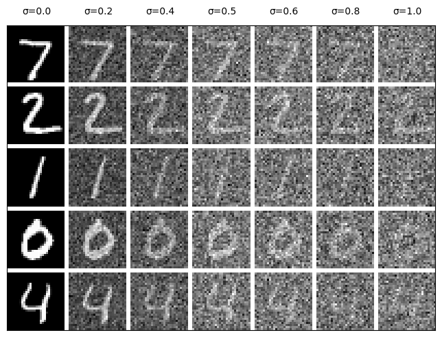
Figure 3: Varying levels of noise on MNIST digits
1.2.1 Training
Now, we will train the model to perform denoising.
- Objective: Train a denoiser to denoise noisy image
- Dataset and dataloader: Use the MNIST dataset via
torchvision.datasets.MNISTwith flags to access training and test sets. Train only on the training set. Shuffle the dataset before creating the dataloader. Recommended batch size: 256. We'll train over our dataset for 5 epochs.- You should only noise the image batches when fetched from the dataloader so that in every epoch the network will see new noised images, improving generalization.
- Model: Use the UNet architecture defined in section 1.1 with
recommended hidden dimension
D = 128. - Optimizer: Use Adam optimizer with learning rate of 1e-4.
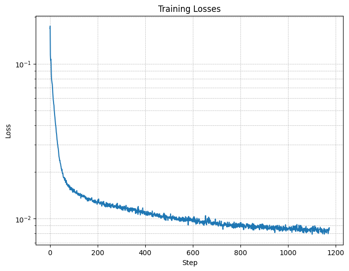
Figure 4: Training Loss Curve
They should look something like these:
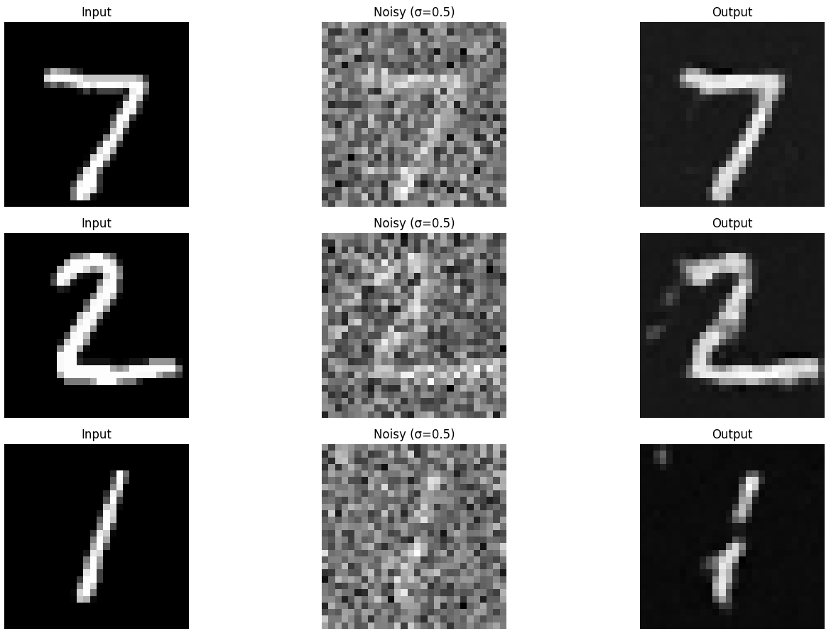
Figure 5: Results on digits from the test set after 1 epoch of training
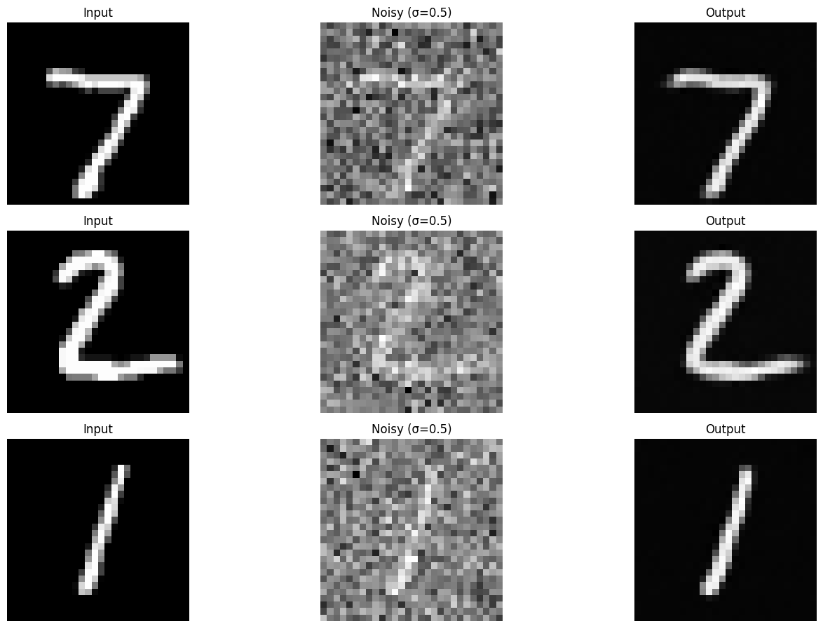
Figure 6: Results on digits from the test set after 5 epochs of training
1.2.2 Out-of-Distribution Testing
Our denoiser was trained on MNIST digits noised with
Visualize the denoiser results on test set digits with varying levels of
noise
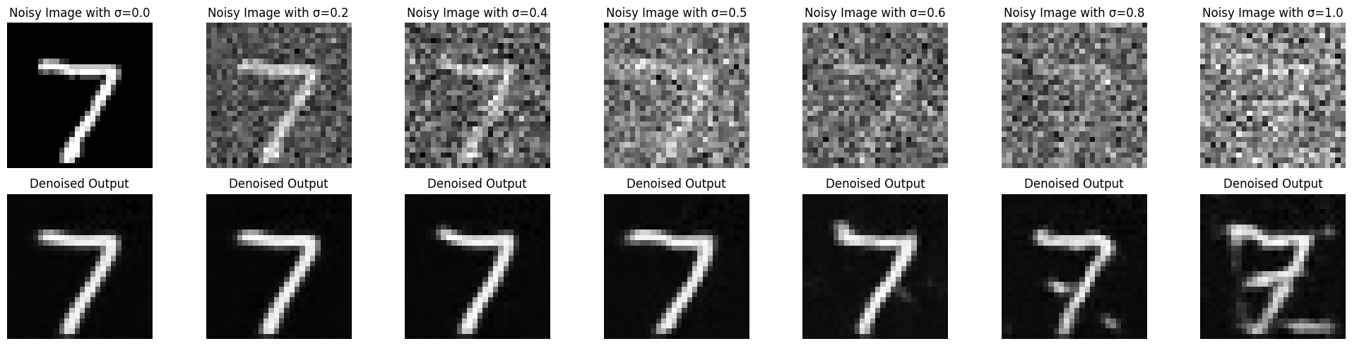
Figure 7: Results on digits from the test set with varying noise levels.
Deliverables
- A visualization of the noising process using
- A training loss curve plot every few iterations during the whole training process (figure 4).
- Sample results on the test set after the first and the 5-th epoch (staff solution takes ~7 minutes for 5 epochs on a Colab T4 GPU). (figure 5, 6)
- Sample results on the test set with out-of-distribution noise levels
after the model is trained. Keep the same image and
vary
- Since training can take a while, we strongly recommend that you
checkpoint your model every epoch onto your personal Google
Drive.
This is because Colab notebooks aren't persistent such that if you are
idle for a while, you will lose connection and your training progress.
This consists of:
- Google Drive mounting.
- Epoch-wise model & optimizer checkpointing.
- Model & optimizer resuming from checkpoints.
Part 2: Training a Diffusion Model
Now, we are ready for diffusion, where we will train a UNet model that can iteratively denoise an image. We will implement DDPM in this part.Let's revisit the problem we solved in equation B.1:
where
For diffusion, we eventually want to sample a pure noise image
Recall in part A that we used equation A.2 to generate noisy images
- Create a list
Now, to denoise image
2.1 Adding Time Conditioning to UNet
We need a way to inject scalar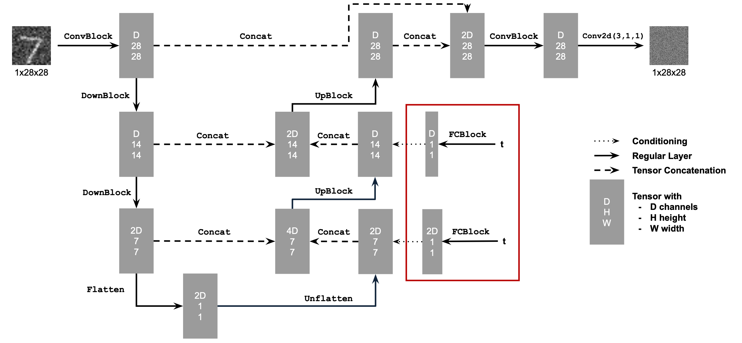
Figure 8: Conditioned UNet
This uses a new operator called FCBlock (fully-connected block) which we use to inject the conditioning signal into the UNet:
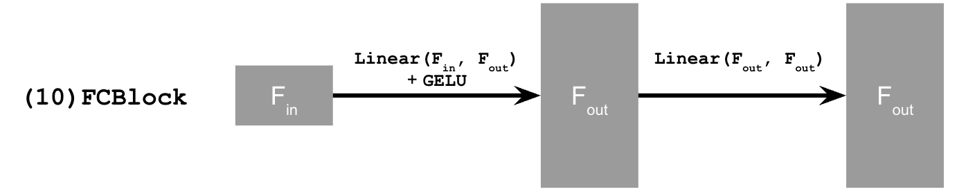
Figure 9: FCBlock for conditioning
nn.Linear.
Since our conditioning signal
You can embed
fc1_t = FCBlock(...)
fc2_t = FCBlock(...)

# the t passed in here should be normalized to be in the range [0, 1]
t1 = fc1_t(t)
t2 = fc2_t(t)

# Follow diagram to get unflatten.
# Replace the original unflatten with modulated unflatten.
unflatten = unflatten + t1
# Follow diagram to get up1.
...
# Replace the original up1 with modulated up1.
up1 = up1 + t2
# Follow diagram to get the output.
...
2.2 Training the UNet
Training our time-conditioned UNet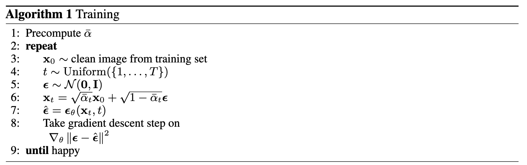
Algorithm B.1. Training time-conditioned UNet
- Objective: Train a time-conditioned UNet
- Dataset and dataloader: Use the MNIST dataset via
torchvision.datasets.MNISTwith flags to access training and test sets. Train only on the training set. Shuffle the dataset before creating the dataloader. Recommended batch size: 128. We'll train over our dataset for 20 epochs since this task is more difficult than part A.- As shown in algorithm B.1, You should only noise the image batches when fetched from the dataloader.
- Model: Use the time-conditioned UNet architecture defined in section 2.1 with
recommended hidden dimension
D = 64. Follow the diagram and pseudocode for how to inject the conditioning signal - Optimizer: Use Adam optimizer with an initial learning rate of
1e-3. We will be using an exponential learning rate decay scheduler with a gamma of
scheduler = torch.optim.lr_scheduler.ExponentialLR(...). You should callscheduler.step()after every epoch.
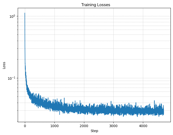
Figure 10: Time-Conditioned UNet training loss curve
2.3 Sampling from the UNet
The sampling process is very similar to part A, except we don't need to predict the variance like in the DeepFloyd model. Instead, we can use our list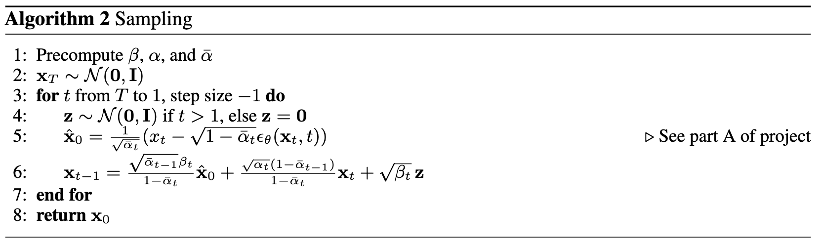
Algorithm B.2. Sampling from time-conditioned UNet
Epoch 1
Epoch 5
Epoch 10
Epoch 15
Epoch 20
Deliverables
- A training loss curve plot for the time-conditioned UNet over the whole training process (figure 10).
- Sampling results for the time-conditioned UNet for 5 and 20 epochs.
- Note: providing a gif is optional.
2.4 Adding Class-Conditioning to UNet
To make the results better and give us more control for image generation, we can also optionally condition our UNet on the class of the digit 0-9. This will require adding 2 more FCBlocks to our UNet but, we suggest that for class-conditioning vector
fc1_t = FCBlock(...)
fc1_c = FCBlock(...)
fc2_t = FCBlock(...)
fc2_c = FCBlock(...)

t1 = fc1_t(t)
c1 = fc1_c(c)
t2 = fc2_t(t)
c2 = fc2_c(c)

# Follow diagram to get unflatten.
# Replace the original unflatten with modulated unflatten.
unflatten = c1 * unflatten + t1
# Follow diagram to get up1.
...
# Replace the original up1 with modulated up1.
up1 = c2 * up1 + t1
# Follow diagram to get the output.
...
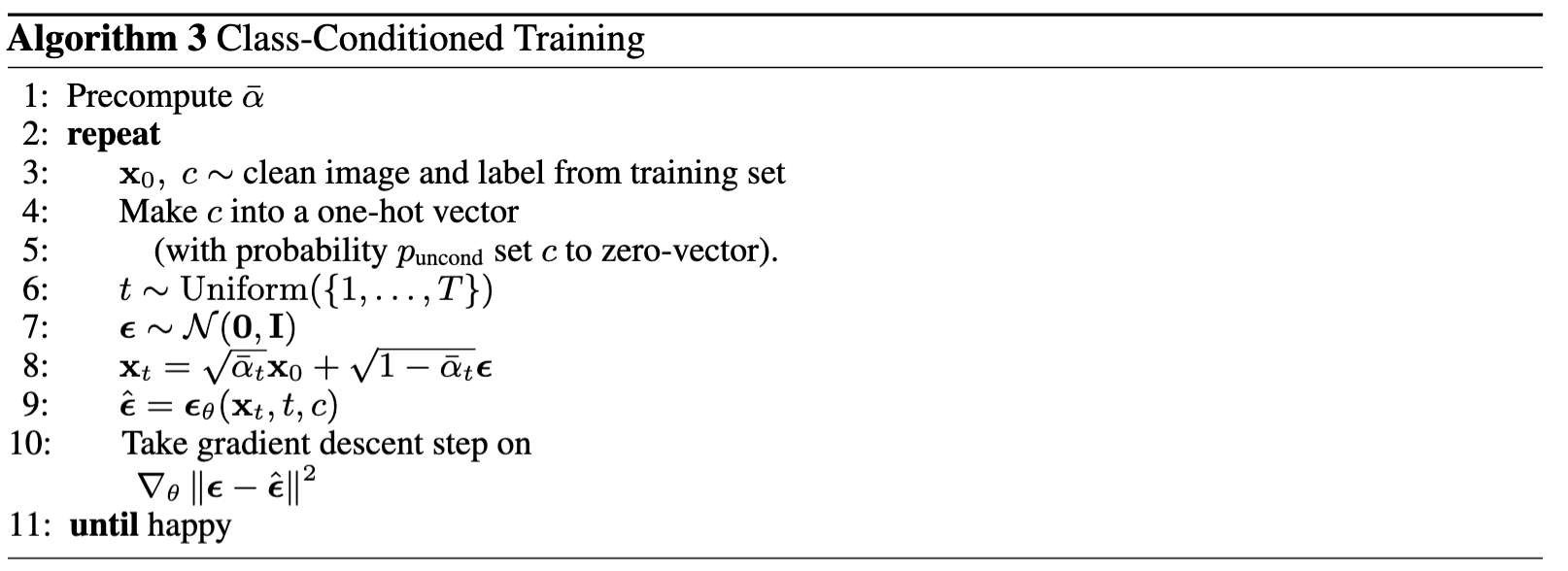
Algorithm B.3. Training class-conditioned UNet
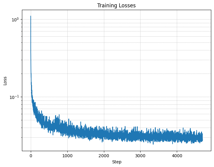
Figure 11: Class-conditioned UNet training loss curve
2.5 Sampling from the Class-Conditioned UNet
The sampling process is the same as part A, where we saw that conditional results aren't good unless we use classifier-free guidance. Use classifier-free guidance with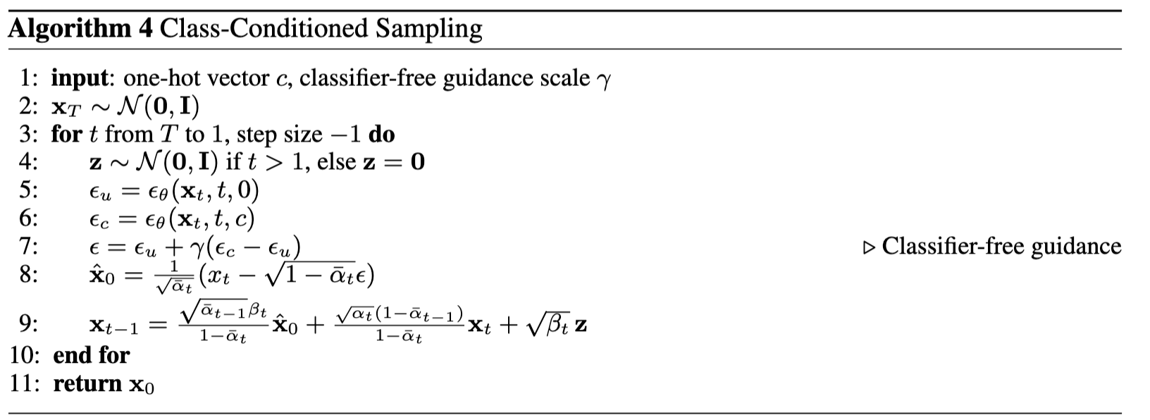
Algorithm B.4. Sampling from class-conditioned UNet
Epoch 1
Epoch 5
Epoch 10
Epoch 15
Epoch 20
Deliverables
- A training loss curve plot for the class-conditioned UNet over the whole training process.
- Sampling results for the class-conditioned UNet for 5 and 20 epochs. Generate 4 instances of each digit as shown
above.
- Note: providing a gif is optional.
Extra Credit
- Improve the UNet Architecture for time-conditional generation
For ease of explanation and implementation, our UNet architecture above is pretty simple. Modify the UNet (e.g. with skip connections) such that it can fit better during training and sample even better results. - Implement Rectified Flow
- Implement rectified flow, which is the state of art diffusion model.
- You can reference any code on github, but your implementation needs to follow the same code structure as our DDPM implementation.
- In other words, the code change required should be minimal: only changing the forward and sample functions.
Acknowledgements
This project was a joint effort by Daniel Geng, Ryan Tabrizi, and Hang Gao, advised by Liyue Shen, Andrew Owens, and Alexei Efros.
Last updated 16 April 2025