CS5625 PA3 Sampling and Filtering
Out: Friday February 26, 2016
Due: Friday March 4, 2016 at 11:59pm
Work in groups of 2.
Overview
In this programming assignment, you will implement:
- antialiased sampling of procedural test patterns,
- high quality reconstruction for scaling of images, and
A few notes on the framework for this assignment:
- There are two applications in the pa3 package, one for each of the two tasks. Each displays a bare-bones UI with just the OpenGL viewport, and an appropriate set of mouse controls to move the images around and explore the aliasing artifacts that result. In the PA_Supersample application, the view deliberately lags behind the mouse, catching up exponentially so that you get slow movement that highlights Moiré patterns.
- Each application makes an attempt to measure its performance and displays three numbers in the corner of the viewport: the duration of time taken to draw the frame, the interval between frames, and the frame rate, which is the reciprocal of the frame interval. These numbers are helpful in understanding how fast your program is running, but they need to be taken with a grain of salt because the Java windowing system takes up a lot of time, especially for large window sizes.
- In order to measure performance, the applications render continuously, which means they will attempt to use all available CPU time. This can be annoying, and if you want a better behaved application when you are not worrying about framerate, you can modify the relevant GLView implementation for your platform, modifying it to use FPSAnimator at 30 or 60 frames per second rather than using the simple Animator class that redraws continuously.
Task 1: Sampling
In this task your job is to implement high-quality antialiased sampling of analytically defined images. One of the images is a test pattern, known as a "zone plate" because of its resemblance to a diffractive optical element of the same name but actually a very simple function: $$f_\text{zp}(x, y) = f_\text{sw}\bigg(\frac{x^2 + y^2}{s^2}\bigg)$$ where $f_\text{sw}$ is a square wave: $$f_\text{sw}(t) = \begin{cases} 0, & t - \lfloor t \rfloor < 0.5 \\ 1, & t - \lfloor t \rfloor >= 0.5 \end{cases}$$ The other test image is a fractal image. The fragment shader that contains all the implementation for this task is patterns.frag.
Point sampling
This part is already done: in point sampling mode, the framework will render either of the patterns, simply evaluating it at the center of each pixel to produce a point-sampled, and highly aliased, result, similar to these images:
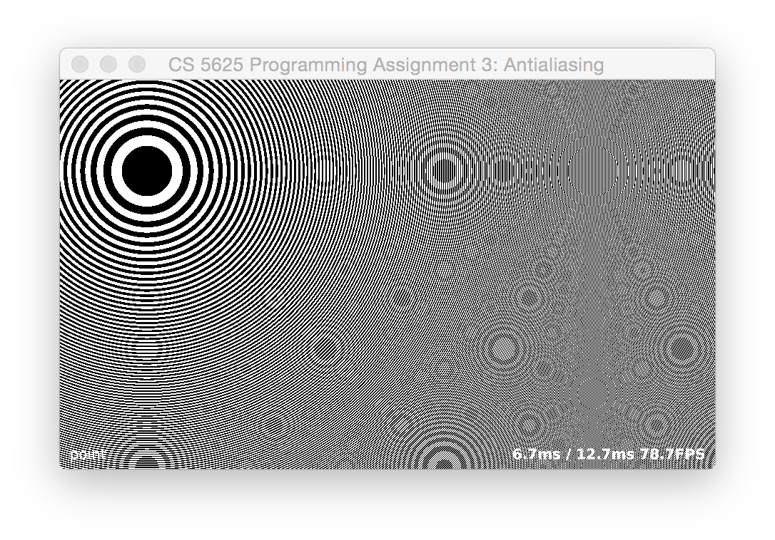 |
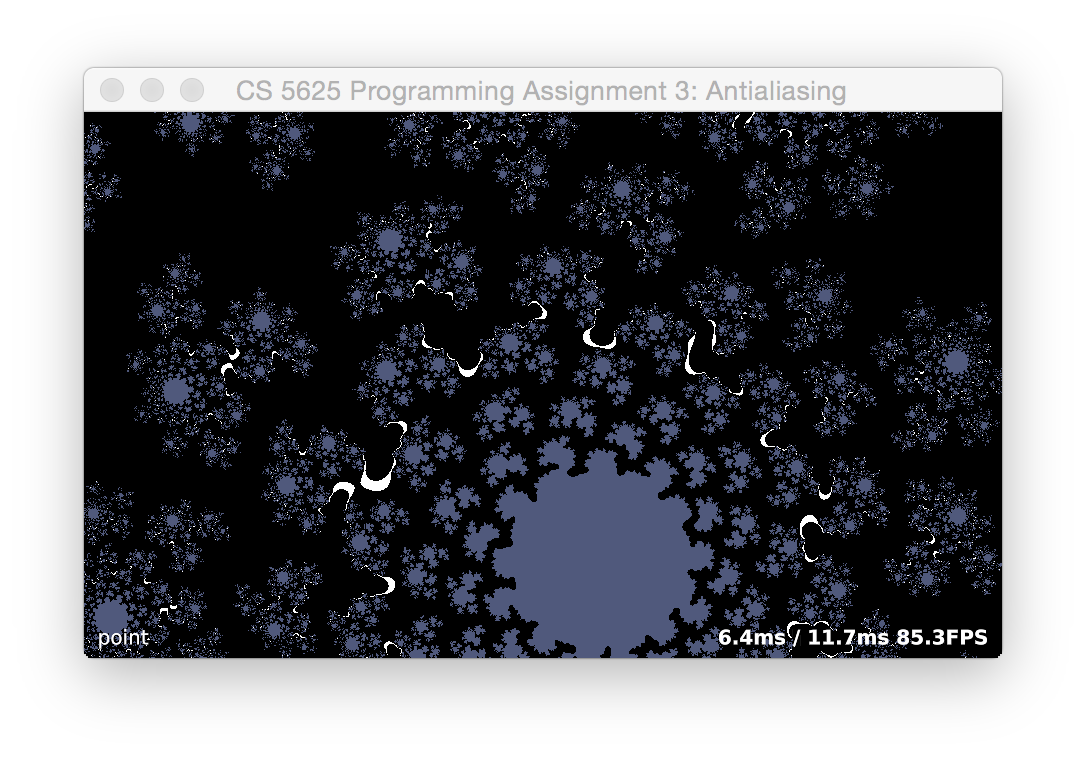 |
There are scale factors in the code called s and fractal_scale that you should feel free to modify based on your screen resolution, so that you can see the broad circles near the origin but also see far enough away to see the patterns that happen near the Nyquist frequency and near the sample frequency. The aliasing from the high contrast, small scale features in the fractal takes the form of shimmering or glittering as the image moves around.
The framework contains the code to draw a full-screen quad with the zoneplate.frag fragment shader, and it passes in a 2D point (controlled by mouse motion) where the center of the pattern should go, and an integer mode, controlled by key presses, that indicates what kind of sampling should be done. MODE_POINT is the default mode that corresponds to this subtask.
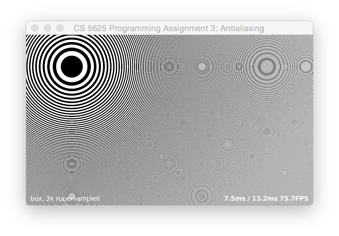
Box filtering with regular supersampling
Once you have point sampling up and running, modify your shader so that when mode is MODE_REGULAR_BOX, for each pixel it averages $N^2$ samples of the same function, positioned in a $N\times N$ grid spread over a unit square (in pixel coordinates) centered at the pixel's sample position. (You can control $N$ using the + and - keys.) Once this is working, you should find that the jaggies on the circles near the center become smooth, and the Moiré patterns are greatly diminshed once $N$ gets to 4 or so, something like this:
 |
 |
(When you're looking at these images, note that your web browser may be layering its own resampling artifacts on top of the ones in the image; open the linked image in its own window to see it more clearly.)
If everything is working right, you should not see the pattern shift as you change $N$; the position of the main bull's-eye should remain the same while the edges get smoother.
Questions to ponder:
- Watch the artifacts produced by the box filter. Why do some artifacts move around when you change the number of samples, but some stay put?
- Which supersampling rates are good at eliminating the artifacts that happen at multiples of the sample frequency?
- What happens in the frequency domain when we approximate a box filter with a grid of samples?
- If you unroll the loop for a fixed value of $N$ does your shader run faster than the general one with for loops?
Box filtering with stochastic supersampling
Some of the artifacts in the previous part—the ones that shift around as you change the sampling rate—are related to the regularity of the supersampling grid. After all, the finer grid has exactly the same problems as the original pixel grid; it just pushes them out to higher frequencies. An alternative, which breaks up grid-related aliasing patterns, is to use random, or stochastic samples. In this task, you approximate the box filtered image, instead of with a regular array of ramples, by using 40 samples placed uniformly and independently within the footprint of the box filter.
Random sampling requires random numbers, and for the purest results they should be uncorrelated from pixel to pixel. Because generating good pseudo-random numbers in shader code is tricky, we have provided a 256x256 texture (unifRandTex) filled with independent random numbers drawn from a uniform distribution over $[0,1]$. Use 80 of these numbers to select the sample locations for each pixel. You want to use different numbers for each pixel; a good way to do this is to use the random() function provided in the shader, which is a classic hack that computes a random-ish hash of a 2D point. Those numbers are not random enough to get excellent results on their own, but if you use that function (seeded with something that varies from fragment to fragment) to select a chunk of random numbers from the texture, you can get nicely uncorrelated samples. (For instance, use the random hash to select the row and the sample index to select the column).
When this part works, you will find many aliasing artifacts disappear, though some, especially around the sample frequency, remain. It also introduces significant noise to the image:
 |
You will want to use texture2DRect to sample these textures using pixel coordinates, as in the second part of this assignment.
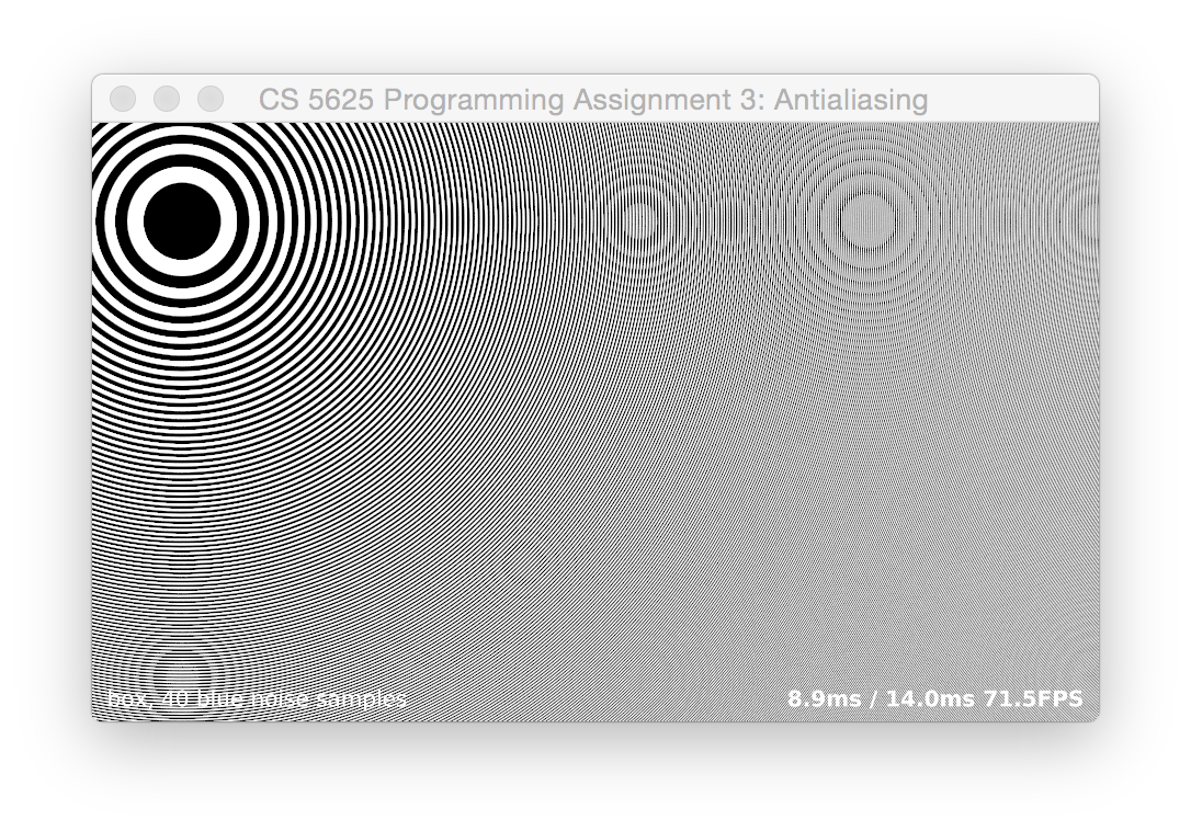
Box filtering with blue noise samples
The noise in random-sampled images can be improved by using samples that are more uniformly distributed than you get by just selecting them independently. Generally speaking, sampling patterns where samples are less likely to be close together or far apart are known as blue noise patterns. The name comes from the Fourier spectra of these patterns, which have less energy at low frequencies (long wavelengths, analogous to red light) and more at high frequencies (short wavelengths, analogous to blue light).
We have provided 256 40-sample blue noise patterns in the unit square, packed into an 80x256 texture. Because blue-noise patterns are not independent samples, it's important to use complete rows of this texture; each row contains a set of 2D coordinates (in the order $x_1, y_1, x_2, y_2, \ldots, x_{40}, y_{40}$) that constitue a nice sampling pattern over the unit square. As before, you'll want to select the rows pseudorandomly to avoid pixel-to-pixel correlations.
You should find the aliasing is quite similar to the independent-random sampling but the noise is noticeably reduced:
 |
Gaussian filtering with stochastic supersampling
With box filtering, things get better with increasing numbers of samples, up to a point, but many of the artifacts are persistent no matter how numerous the samples or how nice their arrangement. We can improve matters by switching to a smoother filter, though at the expense of needing to consider samples over a larger area.
The two ways to approximate the convolution with a filter that has non-constant weights are to use uniformly distributed samples in a weighted average, or to use nonuniformly distributed samples. In this part we will take the second approach, using samples distributed according to a Gaussian probability density $p(x)$. If samples are chosen with this density, and then the sample values are simply averaged, the expected result is $$E\{f(X)\} = \int f(x) p(x) dx.$$ If $p(x)$ is your filter, shifted to the sampling location, then this is the result you are looking for.
We have provided another texture of uniform random numbers, distributed according to a unit-variance Gaussian distribution. They are encoded in the texture so the the value $0$ corresponds to $-3$ (that is, three standard deviations below the mean) and the value $1$ corresponds to $+3$ (three standard deviations above the mean). The tails beyond three standard deviations have been trimmed from the distribution. (To see where all these numbers come from, see the Python and Matlab code in the pa3/textures directory that generates them.)
Add the ability to compute an image sampled using a Gaussian with standard deviation of 0.5 pixels—generally a good compromise between blurring and aliasing—using these Gaussian-distributed samples. You should find that the result further reduces many of the artifacts from the box filter, especially those at high frequencies (for instance, at twice the sample frequency):
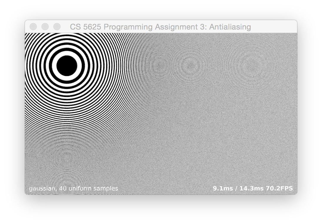 |
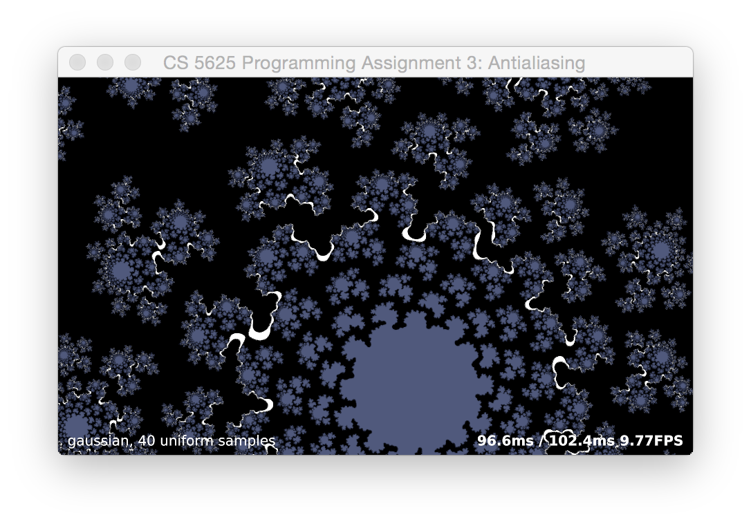 |
How can this behavior be explained by thinking about the Fourier transforms of the box and gaussian filters? Why does the Gaussian do such a good job removing artifacts at, for instance, twice the sample frequency?
Extra challenge: Compute a set of blue-noise sampling patterns that can be used to get the benefits of the gaussian filter but reduce the noise to levels similar to those from the blue-noise box filter.
The Test Application
The test program for this task is implemented in the PA3_Supersample class. You can switch between sampling modes by pressing the following keys:
- p: point sampling
- r: rregularly sampled box filtering
- s: stochastically sampled box filtering
- b: blue noise box filtering
- g: stochastic gaussian filtering
- z: use the zone plate pattern
- f: use the fractal pattern
Task 2: Reconstruction
For the second task, you'll implement several reconstruction filters for enlarging an image in the upsample.frag. The test application for this part, PA3_Upsample, reads in an image and then provides it as a texture to a fragment shader running on a full-screen quad. The texture coordinates are set up to sample from a rectangle in the image—initially, the full image, but you can use the scroll wheel to zoom in and you can click and drag to move the image around on the screen.
There are three filters to implement: box, tent, and cubic. Like the previous task, there is a keyboard-adjustable mode parameter that controls which filter is used. (The keys are listed at the end of this task.) The box corresponds to nearest-neighbor sampling, which happens by itself anyway. The tent corresponds to linear interpolation, similar to what we implemented during lecture. The cubic is a piecewise cubic function with radius of support 2, as described in the SIGGRAPH paper:
D. Mitchell & A. Netravali, “Reconstruction filters in computer graphics,” SIGGRAPH 1988.in Equation 8. Mitchell and Netravali describe a family of cubics with two parameters, $B$ and $C$, and recommend the values $B = C = 1/3$ for general use. Set things up so that it uses those values for MODE_CUBIC_MN; $B = 1, C = 0$ for MODE_CUBIC_BSP; and $B = 0, C = 0.5$ for MODE_CUBIC_CR. The edges of the cactus spikes are quite sharp and need a pretty soft reconstruction to completely eliminate grid artifacts.
A correct implementation looks something like this:
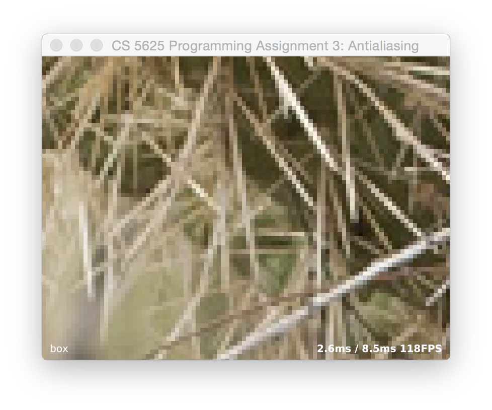
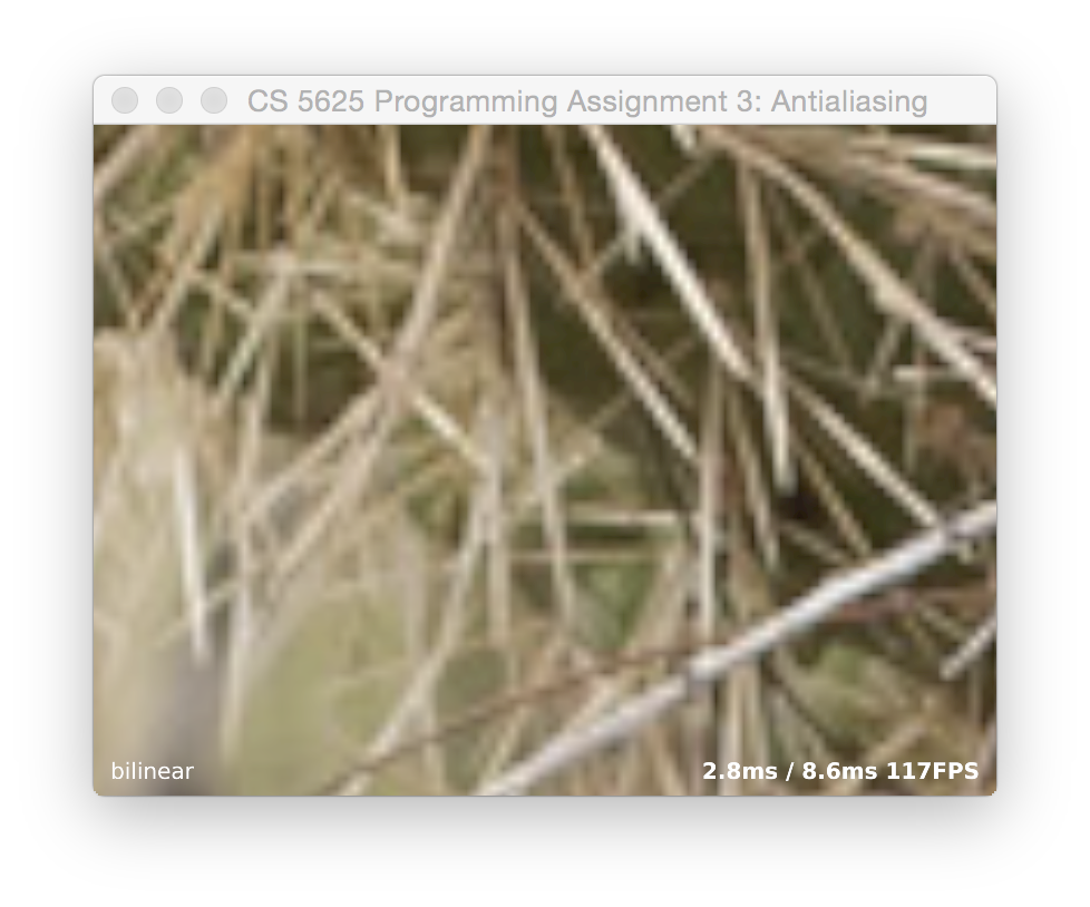
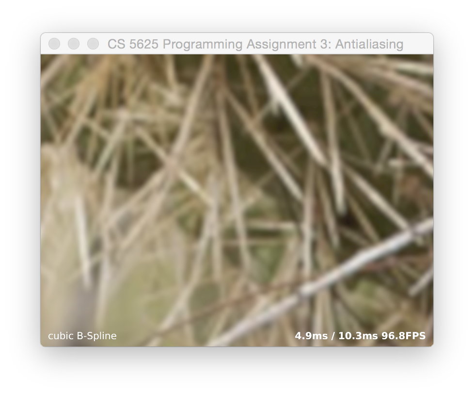
If you have your indexing conventions consistent, the image should not shift around when switching between filters.
Mode Keys
- b: MODE_BOX
- t: MODE_TENT
- c: MODE_CUBIC_CR
- s: MODE_CUBIC_BSP
- m: MODE_CUBIC_MN