CS5625 PA1 Surface Shading

Out: Thursday February 4, 2016

Due: Friday February 12, 2016 at 11:59pm

Work in groups of 2.

Overview

In this programming assignment, you will implement a number of BRDF models. You will also implement an algorithm to compute per-vertex tangent vectors of triangle meshes.

The student folder contains an Eclipse project that contains all the relevant source code. The class pa1.PA1 implements a program that loads and renders three 3D scenes. Running the program, you should see the following window:

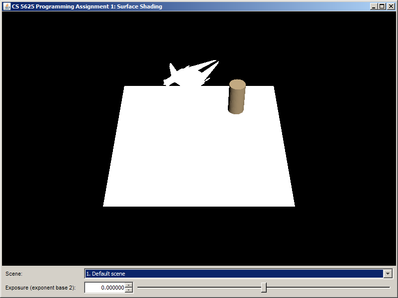
You can use the combo boxes at the bottom of the window to change the scenes and the renderers. The program can be controlled using the following mouse and keyboard combinations:

• LMB or Shift+LMB: Rotating the camera.
• Alt+LMB: Translating the camera view point.
• Ctrl+LMB or Mouse Wheel: Changing the camera zoom.

Task 1: Blinn-Phong Shading Model

In 4620, all real-time assignments used a rendering technique known as “forward” shading, where the lighting and shading of each fragment is computed immediately once the fragment is rasterized from the geometry. Forward shading is implemented in the class pa1.ForwardRenderer. However, we have only provided implemented two types of materials: the "single color" material and the Lambertian one. In this task, we ask you to edit:

• student/src/cs5625/pa1/ForwardRenderer.java
• student/src/shaders/forward/blinnphong.frag

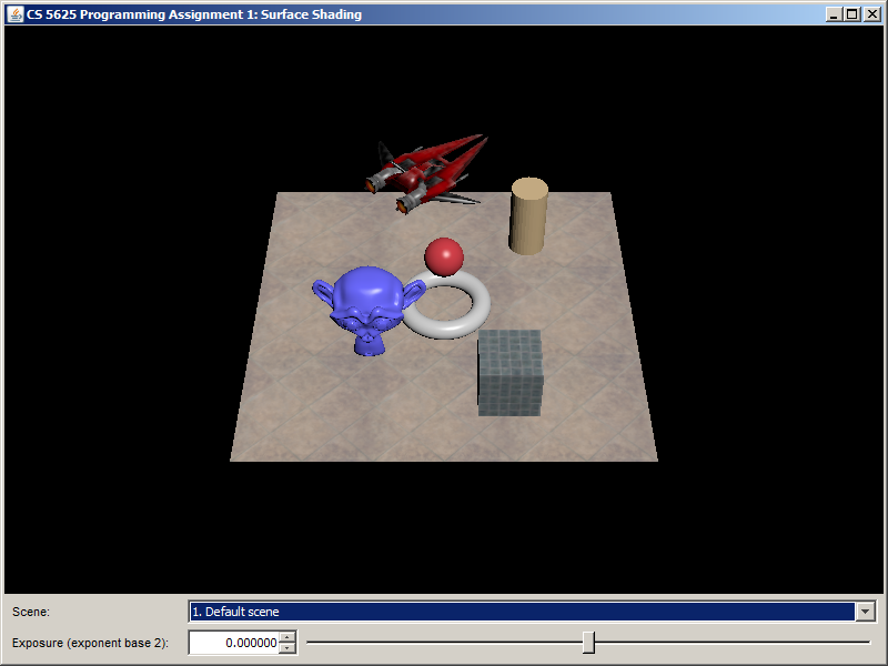
so that the renderer can handle the Blinn-Phong material as well. The Blinn-Phong material itself is implemented by the cs5625.gfx.material.BlinnPhongMaterial class, which you can inspect to see what fields and methods it has. However, you do not need to edit the class itself.

After finishing the implementation, the rendering of the default scene should look like the following:

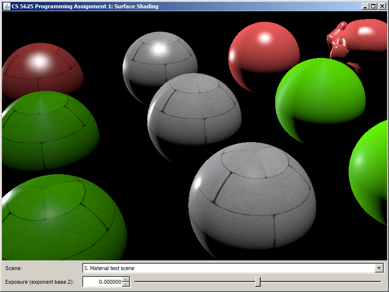
Task 2: Isotropic Microfacet Shading Model

Edit

• PA1/student/src/cs5625/pa1/ForwardRenderer.java
• PA1/student/src/shaders/forward/isotropic_microfacet.frag

to implement the microfacet reflectance model describe in the paper "Microfacet Models for Refraction through Rough Surfaces" by Walter et al., using the GGX model for the normal distribution function (NDF) that was introduced (to graphics) by that paper. (Despite the name, the paper talks about models for both refraction and reflection. However, we will only use the reflection part.)

The parameters of the model are strored in the IsotropicMicrofacetMaterial class, and they are:

• The diffuse color $k_d$ in RGBA format.
• The index of refraction $\eta$, a scalar.
• The roughness parameter $\alpha$, a scalar.

The solution implemented the model as follows. The RGB color of the fragment due to a light source is given by: $$\mathrm{color} = \bigg( k_d + \frac{ F(\mathrm{i}, \mathrm{m}) D(\mathrm{m}) G(\mathrm{i}, \mathrm{o}, \mathrm{m})}{4 | \mathrm{i} \cdot \mathrm{n} | |\mathrm{o} \cdot \mathrm{n} | } \bigg) \max( 0, \mathrm{n} \cdot \mathrm{i} ) \times I$$ where

• $\mathrm{n}$ is the normal vector at the point being shaded,
• $\mathrm{i}$ is the unit vector from the shaded point to the light source,
• $\mathrm{o}$ is the unit vector from the shaded point to the camera,
• $\mathrm{m}$ is half vector between $\mathrm{i}$ and $\mathrm{o}$, in other words, $$\mathrm{m} = \frac{\mathrm{i} + \mathrm{o}}{\| \mathrm{i} + \mathrm{o} \|},$$
• $F(\mathrm{i}, \mathrm{m})$ is the Fresnel factor: $$F(\mathrm{i}, \mathrm{m}) = \frac{1}{2} \frac{(g-c)^2}{(g+c)^2} \bigg( 1 + \frac{(c(g+c)-1)^2}{(c(g-c)+1)^2} \bigg)$$ where $g = \sqrt{\eta^2 - 1 + c^2}$ and $c = |\mathrm{i} \cdot \mathrm{m}|$,
• $D(\mathrm{m})$ is the GGX distribution function: $$D(\mathrm{m}) = \frac{\alpha^2 \chi^+ (\mathrm{m} \cdot \mathrm{n})}{\pi \cos^4 \theta_m (\alpha^2 + \tan^2 \theta_m)^2}$$ where $\chi^+$ is the positive characteristic function ($\chi^+(a) = 1$ if $a> 0$ and $\chi^+(a) = 0$ if $a \leq 0$), and $\theta_m$ is the angle between $\mathrm{m}$ and $\mathrm{n}$,
• $G(\mathrm{i}, \mathrm{o}, \mathrm{m})$ is the shadowing-masking function of the GGX distribution: $$G(\mathrm{i}, \mathrm{o}, \mathrm{m}) = G_1(\mathrm{i},\mathrm{m}) G_1(\mathrm{o}, \mathrm{m})$$ and $$G_1(\mathrm{v},\mathrm{m}) = \chi^+((\mathrm{v} \cdot \mathrm{m}) (\mathrm{v} \cdot \mathrm{n})) \frac{2}{1 + \sqrt{1 + \alpha^2 \tan^2 \theta_v}}$$ where $\theta_v$ is the angle between $\mathrm{v}$ and $\mathrm{n}$.
• $I$ is the "power" of the light source. See more details on how the power is computed in the implementation details section.

Task 3: Tangent space computation

When shading with an anisotropic model or computing normals from a tangent-space normal map, a complete orthogonal coordinate system at the shaded point is needed. This means we need to define two orthogonal vectors perpendicular to the surface normal at each point on the surface—these vectors span the tangent space to the surface at that point, and together with the normal vector, $\mathrm{n}$, they are often called the tangent frame.

It's important to have a consistent way to choose these tangent vectors, and the usual way is to define them based on the texture coordinates. Let the first tangent vector, $\mathrm{t}$, called just the “tangent,” point in the direction that the first texture coordinate, $u$, increases (so that it's tangent to the lines of constant $v$), and let the second tangent vector, $\mathrm{b}$, called the “bitangent,” complete a right-handed orthonormal basis.

In this task, edit the computeTriMeshTangents method of the TriMeshUtil class to compute the tangent space at each vertex of a triangle mesh according to the algorithm given in this web page. Be sure to appropriately cite this source in your code.

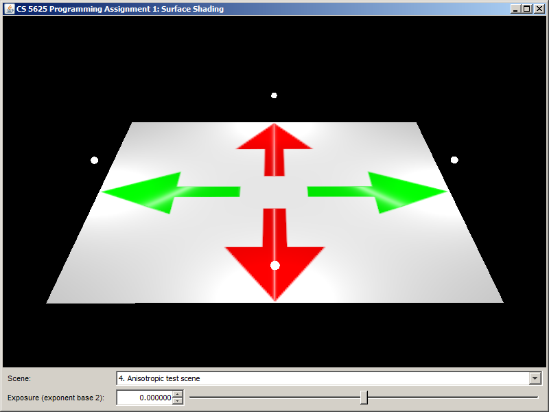
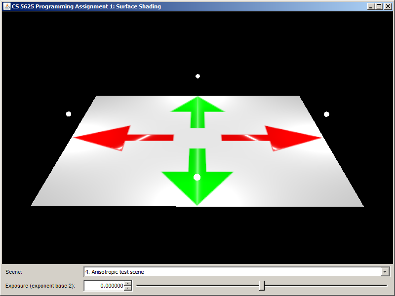
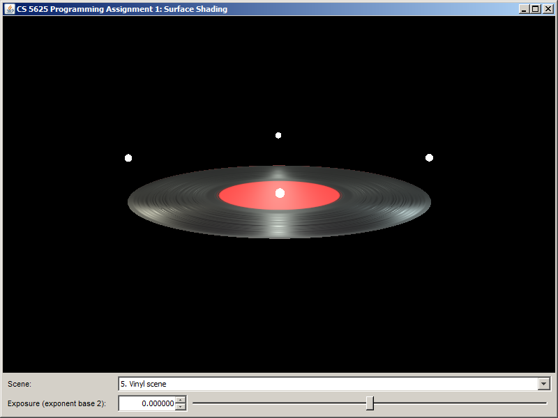
Task 4: Anisotropic Microfacet Shading Model

With the tangent space computed, you are now ready to implement the anisotropic version of the microfacet shading model. For an anisotropic surface, the NDF is no longer a function only of the angle between the normal and the half vector, but depends on the components of the half vector in the $\mathrm{t}$ and $\mathrm{b}$ directions independently. The model we'll use is almost the same as the isotropic one. The only differences are in $D$ and $G_1$, which must now be calculated using the tangent space and two roughness parameters $\alpha_X$ and $\alpha_Y$, specificed separately to indicate the width of the NDF in the direction of $\mathrm{t}$ and $\mathrm{b}$ respectively.

Consider the coordinate frame with the tangent $\mathrm{t}$ as its x-axis, the bitangent $\mathrm{b}$ as its y-axis, and the surface normal $\mathrm{n}$ as its z-axis. Let $m_t$, $m_b$, and $m_n$ be the scalars such that $$\mathrm{m} = m_t \mathrm{t} + m_b \mathrm{b} + m_n \mathrm{n}.$$ (Note that $m_n = \mathrm{m} \cdot \mathrm{n} = \cos \theta_m$, $m_t = \mathrm{m} \cdot \mathrm{t}$, and $m_b = \mathrm{m} \cdot \mathrm{b}$.) Then, the anisotropic version of the GGX distribution is given by: $$D(\mathrm{m}) = \frac{\chi^+(\mathrm{m} \cdot \mathrm{n})}{ \pi \alpha_X \alpha_Y \bigg(m_n^2 + \frac{m_t^2}{\alpha_X^2} + \frac{m_b^2}{\alpha_Y^2} \bigg)^2}.$$ (See if you can show that the above expression is the same as the definition of $D$ in Task 2 when $\alpha_X = \alpha_Y$.) The shadow masking function $G$ is the same as that of the isotropic function, except that the roughness parameter $\alpha$ must be calculated from $\alpha_X$ and $\alpha_Y$ as follows: $$\alpha = \sqrt{\frac{\alpha_X^2 m_t^2 + \alpha_Y^2 m_b^2}{m_t^2 + m_b^2} }.$$

Edit

• PA1/student/src/cs5625/pa1/ForwardRenderer.java
• PA1/student/src/shaders/forward/anisotropic_microfacet.frag

to put the above formulas into action. After completing this exercise, the rendering of the "material test" scene (3rd scene in the combo box) should look like the image below.

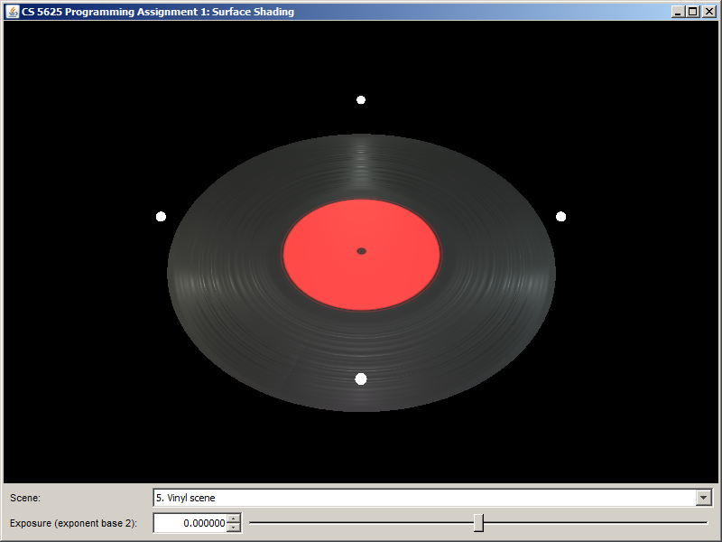
We also provide two test scenes: the ``anisotropic test scene" and the "vinyl scene". The renderings produced by the solution systems of the three test scenes are given below:

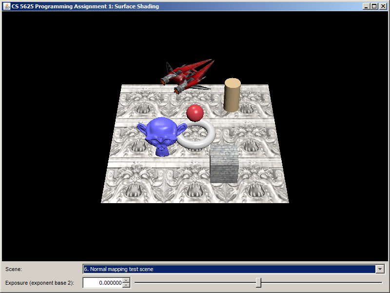
Task 5: Tangent-Space Normal Mapping

Edit:

• PA1/student/src/cs5625/pa1/ForwardRenderer.java
• src/shaders/forward/normalmap_blinnphong.frag

so that the forward renderer implements a Blinn-Phong shading model together with a tangent space normal map. The only difference between this model and the standard version is how the normal at the shaded point is computed. In the standard version, we just normalize the vector given to us through the varying variable geom_normal. In this version, however, we first need to compute an orthonormal tangent space at the shaded point and then use it, together with the texture value of the normal map, to compute the effective normal.

Let us first discuss the computation of the tangent space. The vertex shader will pass three varying variables: geom_normal, geom_tangent, and geom_bitangent to the fragment shader. The vectors contained in these variabled are interpolated from those same vectors at the vertices. Hence, they are not necessarily orthonormal or even normalized. To recover, an orthonomal frame ($\mathbf{t}$, $\mathbf{b}$, $\mathbf{n}$), we suggest that you:

1. Normalize the geom_normal variable to get the normal vector $\mathbf{n}$.
2. Project geom_tangent to the plane perpendicular to $\mathbf{n}$ and then normalize it to get $\mathbf{t}$.
3. Compute the cross product $\tilde{\mathbf{b}} = \mathbf{n} \times \mathbf{t}$.
4. If the dot product between geom_bitangent and $\tilde{\mathbf{b}}$ is greater than 0, set $\mathbf{b} = \tilde{\mathbf{b}}$. Otherwise, set $\mathbf{b} = -\tilde{\mathbf{b}}$.

In other words, we want a frame where the normal is parallel to the interpolated value. The tangent vector is as close as possible to the interpolated value but perpendicular to the normal. The bitangent is "redefined" to be parallel to the cross product between $\mathbf{n}$ and $\mathbf{t}$, but pointing in the direction that preserves the handedness given by the original mesh data.

Next is the computation of the effective normal. The normal map encodes the normal texture as a color as follows: $$\begin{bmatrix} r \\ g \\ b\end{bmatrix} = \begin{bmatrix} (\bar{\mathbf{n}}_x + 1) /2 \\ (\bar{\mathbf{n}}_y + 1) /2 \\ (\bar{\mathbf{n}}_z + 1) /2 \end{bmatrix}$$ where $\bar{\mathbf{n}} = (\bar{\mathbf{n}}_x, \bar{\mathbf{n}}_y, \bar{\mathbf{n}}_z)^T$, in tangent space, being encoded. You should recover the tangent space normal from the color of the texture at the shaded point. Then, the effective normal $\mathbf{n}_{\mathrm{eff}}$ is given by: $$\mathbf{n}_{\mathrm{eff}} = \bar{\mathbf{n}}_x \mathbf{t} + \bar{\mathbf{n}}_y \mathbf{b} + \bar{\mathbf{n}}_z \mathbf{n}.$$ Proceed by using the effective normal to shade the fragment.

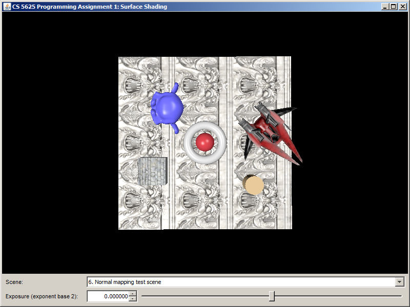
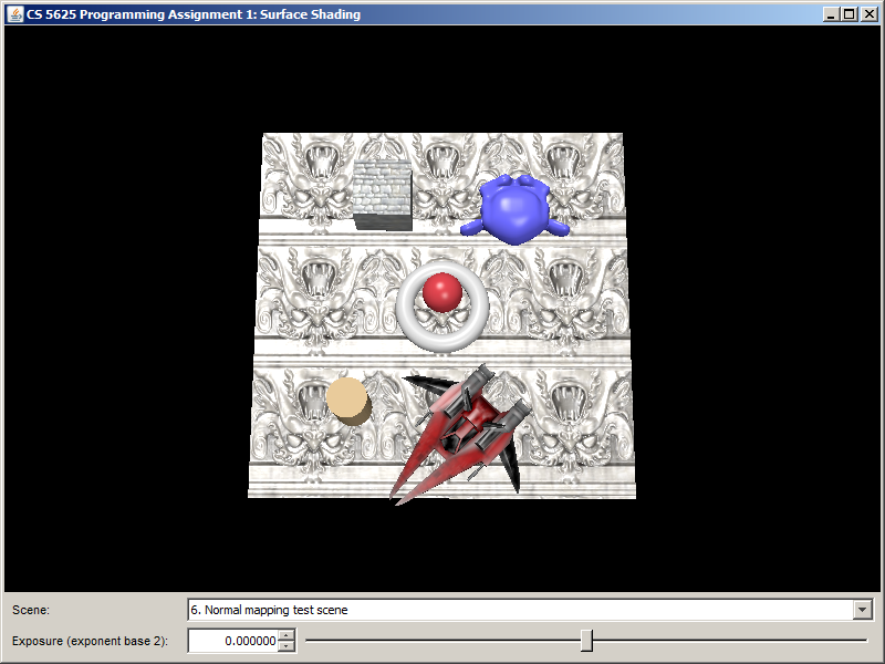
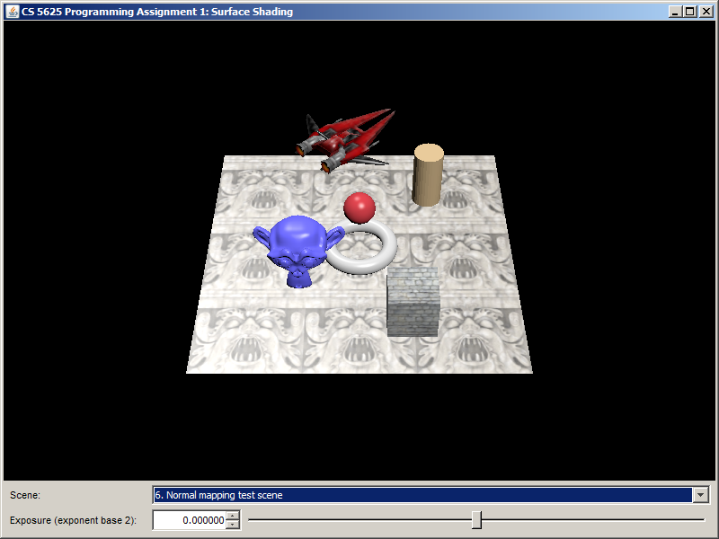
After implementing the shader, the floor and the cube in the "normal mapping test" scene should become much more interesting:

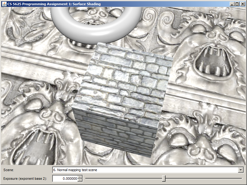On the other hand, here is what it would look like if the ground plane and the cube are shaded with standard Blinn-Phong model.

You can see that normal mapping provides more surface details.

The following are renderings produced by the solution system of the "tangent test scene."

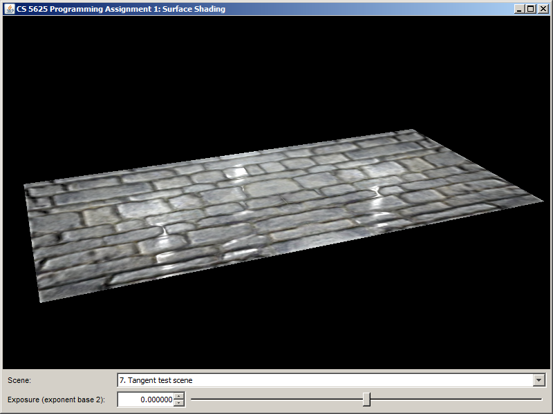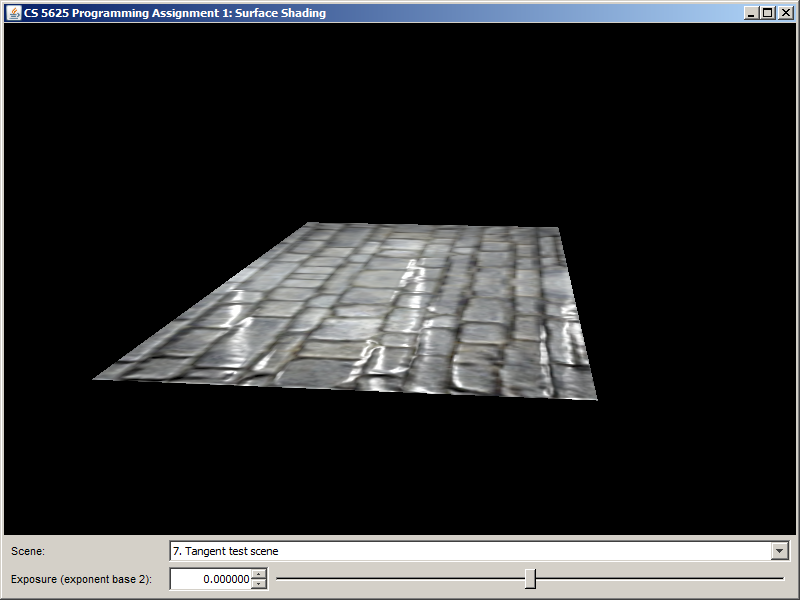Requirements

The framework for programming assignments was written in Java 8. It does not run on older (or netbook) hardware. Known requirements are:

1. The GPU must support OpenGL 2.1 and GLSL 1.3.
2. The GPU must support the GL_ARB_texture_rectangle extension.
3. The GPU must support at least 4 color attachments on a frame buffer object.
4. The GPU must support at least 5 texture targets.
5. The GPU must suport dynamic branches and loops in fragment shaders.

All Gates Hall lab computers have up-to-date GPUs and should be able to run the framework without problems.

What to Submit

You should submit a ZIP file containing all the source codes and data in the PA1/student directory. All the code you have written should be well commented and easy to read, and header comments for all modified files should appropriately indicate authorship. Be sure to cite sources for any code or formulas that came from anywhere other than your head or this assignment document. Also, put in the directory a readme file explaining any implementation choices you made or difficulties you encountered.

Implementation Details

Use of Textures

Some material properties are stored as a scalar/vector value and a texture. For example, in the BlinnPhongMaterial class, there is both the specularColor field and teh specularTexture field. In such a case, the scalar/vector value must be defined, but the texture can be left unspecified (i.e., null).

In the corresponding fragment shader, there will be 3 uniforms related to the material parameter. One uniform corresponds to the scalar/vector value (for example, mat_specular). One uniform serves as a flag telling whether there exists the corresponding texture (for example, mat_hasSpecularTexture). One uniform corresponds to the texture (for example, mat_specularTexture). If the texture is undefined, you should use the scalar/vector value to calculate shading. If the texture is undefined, you should fetch the texture value, multiply it with the scalar/vector value, and use the product to compute shading. For example, we might compute the specular value that will used later for shading in the fragment shader as follows:

vec3 specular = mat_specular;
if (mat_hasSpecularTexture) {
  specular *= texture2D(mat_specularTexture, geom_texCoord).xyz;
}

Point Light Sources

Light sources in this PA are all point light sources and implemented in the PointLight class. A point light is specified by three parameters: its position, its color (i.e., power), and its 3 attenuation coefficients. The power reaching a shaded point is computed in a non-physical manner as follows: $$\mathrm{power} = \frac{color}{A + Bd + Cd^2}$$

where $d$ is the distance between the light source and the shaded point, $A$ is the constant attenuation coefficient, $B$ is the linear attenuation coefficient, and $C$ is the quadratic attenuation coefficient. You can see this calculation implemented in the fragment shader of the lambertian material.