CS5625 PA Shadows
Out: Thursday April 9, 2015
Due: Thursday April 23, 2015 at 11:59pm
Work in groups of 2.
Overview
In this assignment, you will implement 4 techniques for simulating shadows in interactive graphics application:
- vanilla shadow mapping,
- shadow mapping with percentage closer filtering (PCF),
- shadow mapping with percentage closer soft shadows (PCSS), and
- screen-space ambient occlusion (SSAO).
Task 1: Porting Your Own Code from PA1
For convenience, we will use the deferred shader which was used back in PA1. Since this assignment focuses on shadows and not shading models, we will only use the Lambertian and Blinn-Phong shading model. First, edit:
so that they pass the right information to the übershader. However, make sure that the eye-space position of the fragment must be stored in the first three components of the 3rd G-Buffer, so that your shaders work with the new übershader in this PA. Then, modify
So that the übershader shades the Lambertian and Blinn-Phong models correctly. Notice that, when the übershader shades a fragment of the two models, it splits into two cases based on whether spotLight_enabled is true or not. If the variable is false, you should use the point lights to shade the pixels like in PA1. Otherwise, you should use the parameters of the spot light (stored in spotLight_color, spotLight_attenuation, and spotLight_eyePosition) to shade the fragment. You will also find that in the latter case, the shadowing factor is computed and stored in the factor variable. You should multiply this factor with spotLight_color before shading with the spot light before shading so that the light can be properly shadowed in the next tasks.
Task 2: Shadow Map Generation
In this programming assignment, we will implement spot lights whose illumination area is a rectangle. The spot light is represented by the ShadowingSpotLight class. As you will see from the code, the spot light contains a perspective camera within it. The rectangular cone emanating from the camera's eye position represents the space that can be lit by the spot light. The first step to implement the spot light is to generate the shadow map, which is basically a rendering of the scene from the point of view of this camera.
Edit
so that the shader writes the appropriate information into the shadow map.The shader contains the following uniforms and varying variables:
- geom_position: the eye-space position (with respect to the camera of the light) of the fragment.
- sys_projectionMatrix: the projection matrix of the light's camera.
- shadowMapWidth and shadowMapHeight: the width and height of the shadow map, respectively.
The information that needs to be written into the shadow map is determined by the needs of the shadow mapping shader that will read from this map and compute a shadow factor to be used in shading. That code needs to know the distance from the light to the nearest surface, and it also needs access to derivative information about this distance, to be used in computing slope-dependent shadow bias.
Let us call the above eye-space position $\mathbf{p}''$. The normalized device coordinate before the perspective divide is computed as $P\mathbf{p}'$ where $P$ denotes sys_projectionMatrix. Let $\mathbf{p}'$ denote $P\mathbf{p}''$. Recall that the depth of the fragment (that is used for depth testing and shadow mapping) is given by $\mathbf{p}'.z / \mathbf{p}'.w$. Because $P$ represents perspective projection, $\mathbf{p}'.w = -\mathbf{p}''.z$.
Because we will make use of both the depth afer perspective divide (Task 3) and the $z$-coordinate before the perspective divide (Task 5), you need to write both the $z$-component and the $w$-component of $\mathbf{p}'$ to the shadow map. More specifically, if we let $\mathbf{q}$ denote the output fragment color of the shadow map (i.e., gl_FragColor), then set: \begin{align*} \mathbf{q}.z &:= \mathbf{p}'.z \\ \mathbf{q}.w &:= \mathbf{p}'.w \end{align*}
To implement slope-dependent bias, we need the screen space derivative of the depth $\mathbf{p}'.z/\mathbf{p}'.w$. By using the dFdx and dFdy functions with geom_position, you can compute $\partial \mathbf{p}''/\partial x$ and $\partial \mathbf{p}''/\partial y$. Using these values and some basic calculus, you can compute $\partial (\mathbf{p}'.z / \mathbf{p}'.w) / \partial x$ and $\partial (\mathbf{p}'.z / \mathbf{p}'.w) / \partial y$. However, these partial derivatives actually depend on the size of the shadow map. (That is, if the shadow map is 2 times bigger in each dimension, the partial derivative will be 2 times smaller in magnitude.) To make the derivatives scale independent, you should multiply them with the side lengths of the shadow map. In effect, write these quantities to the $x$- and $y$-component of gl_FragColor: \begin{align*} \mathbf{q}.x &:= \frac{\partial (\mathbf{p}'.z / \mathbf{p}'.w)}{\partial x} \times \mathtt{shadowMapWidth} \\ \mathbf{q}.y &:= \frac{\partial (\mathbf{p}'.z / \mathbf{p}'.w)}{\partial y} \times \mathtt{shadowMapHeight} \end{align*}
You can visualize the shadow map by selecting the "Shadow Map" display mode. The shader for this mode displays the $w$-component of the shadow map pixels in such a way that the value specified by the "Shadow Map Min Z" is displayed as black and the value specified by the "Shadow Map Max Z" is displayed as white.
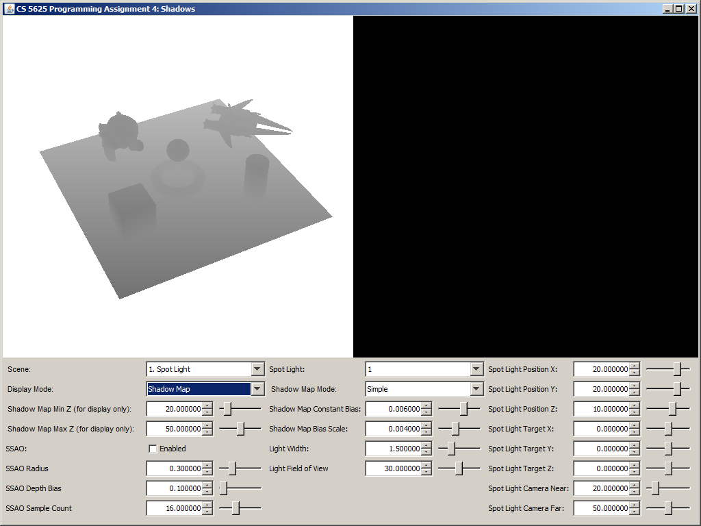
A visualization of the shadow map of the "Spot Light" scene.
Task 3: Shadow Mapping
Edit
- the appropriate branch of the getShadowFactor function in student/src/shaders/deferred/ubershader.frag
Your implementation should make use of the following uniforms in the shader:
- spotLight_shadowMap: the shadow map.
- spotLight_shadowMapWidth: the width, in pixels, of the shadow map.
- spotLight_shadowMapHeight: the height, in pixels, of the shadow map.
- spotLight_viewMatrix: the view matrix of the light's camera.
- spotLight_projectionMatrix: the projection matrix of the light's camera.
- spotLight_shadowMapConstantBias: the constant shadow map bias.
- spotLight_shadowMapBiasScale: the multiplicative factor for the slope-dependent shadow map bias.
The getShadowFactor should return a floating point number whose value ranges from $0$ to $1$, where the value represents that fraction of light energy that reaches the point being shaded. The value $1$ means the shaded point receives all the light energy, and the value $0$ means the shaded point is completely in shadow. The function takes one argument, called position, which is the position of the point being shaded, retrieved from the G-Buffer. As such, this position is in the eye-space of the camera that is used to render the scene. Obviously, this camera is not the same as the one used to render the shadow map.
You shader should transform position to a texture coordinate of the shadow map. This involves first undoing the effect of the main camera's view transformation, which you can use the sys_inverseViewMatrix to do so. You should then transform the result with spotLight_viewMatrix and spotLight_projectionMatrix. Let us call the resulting 4D point $\mathbf{p}$. To get the texture coordinate, perform the perspective divide and then multiply with the appropriate scaling factors in the $x$ and $y$ components. Use result to read from the shadow map, and let us call the result $\mathbf{q}$. Recall from the last task that: \begin{align*} \mathbf{q}.x &= \frac{\partial (\mathbf{q}.z / \mathbf{q}.w)}{\partial x} \times \mathtt{shadowMapWidth} \\ \mathbf{q}.y &= \frac{\partial (\mathbf{q}.z / \mathbf{q}.w)}{\partial y} \times \mathtt{shadowMapHeight} \\ \mathbf{q}.w &= -\mathbf{p}''.z. \end{align*} where $\mathbf{p}''$ is point closest to the light (but farther than the shadow map's near plane) on the ray from the light source position to $\mathbf{p}$. Moreover, the $z$-component of the normalized device coordinate (i.e., the depth) is given by $\mathbf{q}.z / \mathbf{q}.w$.
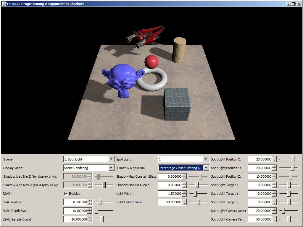
In this task, the getShadowFactor should only output either $0$ or $1$ (i.e., the point is either entirely in shadow or not at all under shadow). The point is under shadow if and only if: $$ \frac{\mathbf{p}.z}{\mathbf{p}.w} > \frac{\mathbf{q}.z}{\mathbf{q}.w} + \mathtt{spotLight\_shadowMapBiasScale} \times \max ( |\mathbf{q}.x|, |\mathbf{q}.y| ) + \mathtt{spotLight\_shadowMapConstantBias}.$$
A correct implementation of the shader should yield the following pictures.
 |
 |
 |
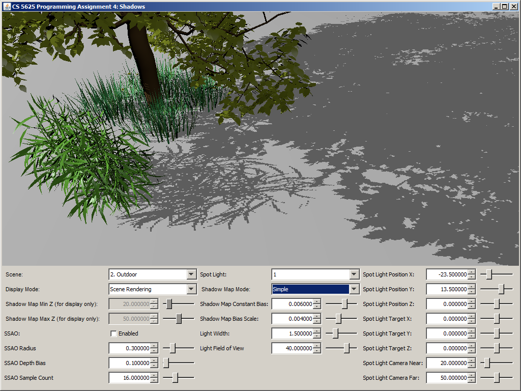 |
You should play with the constant bias and the slope-dependent bias factor to see its affect. In general, as you increase either bias, less of the scene should be in shadow. Also, if you set both parameters to zero, you should see lots of shadow acne.
Task 4: Percentage Closer Filtering
Edit
- the appropriate branch of the getShadowFactor function in student/src/shaders/deferred/ubershader.frag
Your implementation should make use of the following uniforms in the shader:
- spotLight_pcfKernelSampleCount: the number of samples to use for this task.
- spotLight_pcfWindowWidth: the side length of the square window in the shadow map to sample from.
According to original PCF paper (Reeves et al.), one should take a pixel footprint in screen space, project this footprint into the shadow map, and sample shadow map points in this area. However, the GPU Gems article advises doing away with the aforementioned transformation. That is, we basically form a square window of size spotLight_pcfWindowWidth around the shadow map position, which is the position parameter to the getShadowFactor function. From this window, you should sample spotLight_pcfKernelSampleCount points using the shadow mapping algorithm from the last task, compute the fraction of samples whose depth (after incorporating bias) is less than position's depth, and output this fraction as the shadow factor.
We advise that you generate the sample points by using a prefix of the list of Poisson disc samples that you used in PA3. (If spotLight_pcfKernelSampleCount is more than 40, you can clamp it to 40.) To remove banding artifacts, you should also apply a random rotation to the point set too.
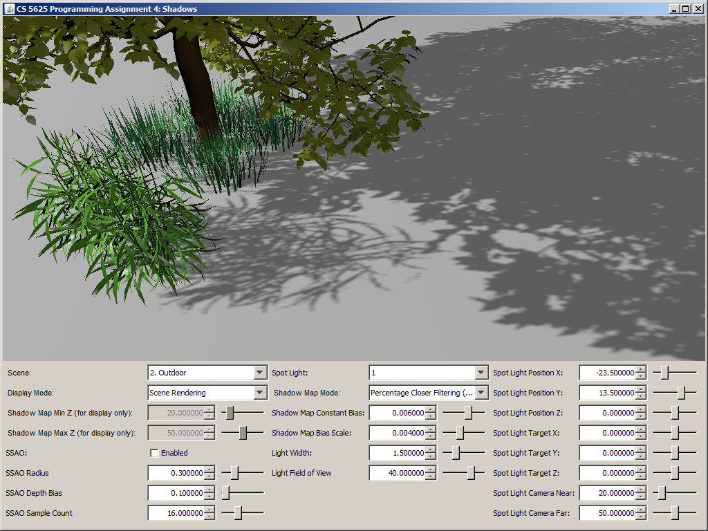
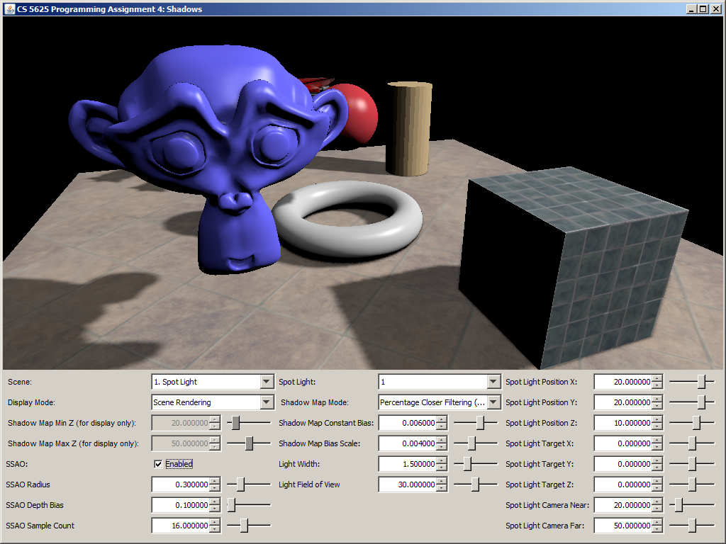
A correct implementation should yield the following images:
| No PCF | With PCF |
|
 |
|
 |
|
 |
|
 |
Task 5: Percentage Closer Soft Shadows
Edit
- the appropriate branch of the getShadowFactor function in student/src/shaders/deferred/ubershader.frag
Your implementation should make use of the following uniforms in the shader:
- spotLight_lightWidth: the 1D width of the light source in scene unit. The light source is a square whose size is of length spotLight_lightWidth centered at the point $(0,0,0)$ and lying in the $xy$-plane in the eye-space of the light source's camera.
- spotLight_pcssBlockerKernelSampleCount: the number of samples to use when computing the average blocker depth.
- spotLight_pcssPenumbraKernelSampleCount: the number of samples to use when actually computing the shadow factor.
As you probably have read in the document, the first step of PCSS involves estimating the area in which you will sample the shadow map for depths of blockers. To do this, compute the length of the side of the light source if it were to be projected onto the near plane of the light source's camera. You will find that the spotLight_near and spotLight_fov are useful for this calculation. Let us denote the computed size by $s$, and let the unit of $s$ be shadow map pixels.
Next, you should sample spotLight_pcssBlockerSampleCount points from the shadow map in the square of side length $s$ around the point on the shadow map which corresponds to the position argument of the getShadowFactor function. The samples can be generated using the Poisson disc points like what you did in the last task. You should find the average of the $z$-coordinate of the samples that pass the shadow map test. Recall that Task 2 directs you to store the (negative of the) $z$-coordinate of the geometry in the $w$-component of the shadow map texel. This is the value that should be used to compute the average blocker depth.
After getting the average $z$-coordinate of the blocker, you should use it to find the penumbra size as specified in the Fernando's paper. Use this penumbra size as the window size, evaluate PCF shadow factor with spotLight_pcssPenumbraKernelSampleCount samples, and return the result as the shadow factor for PCSS.
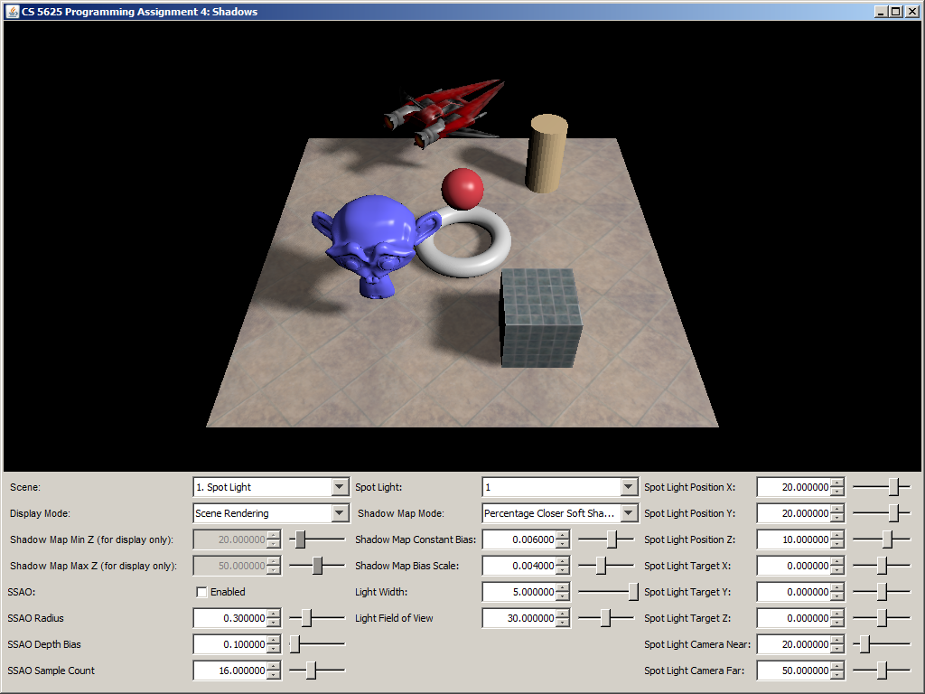
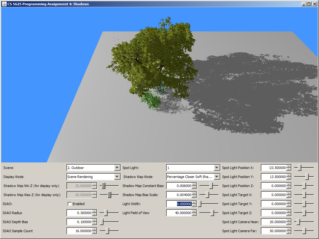
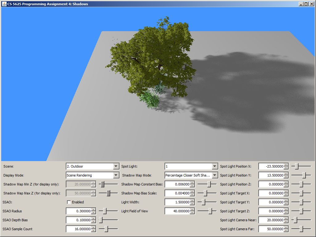
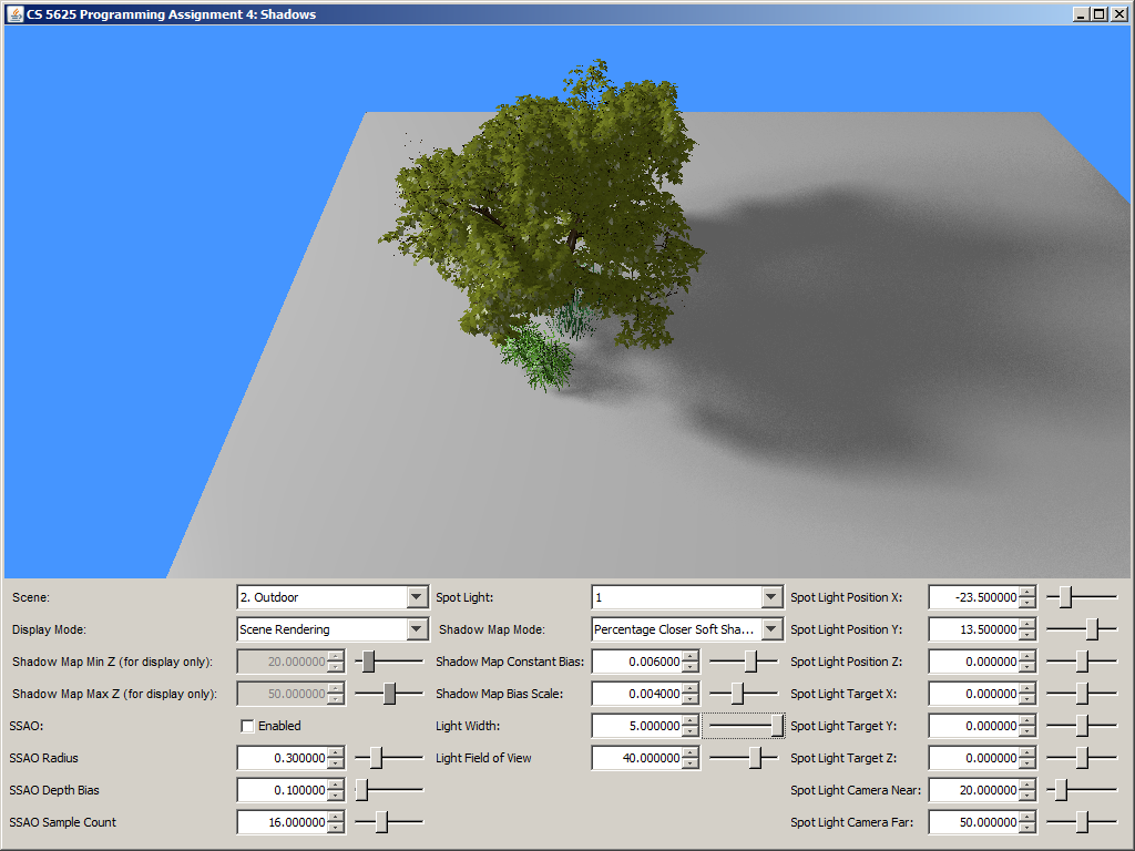
A correct implementation should yield a picture that looks like simple shadow mapping when the light width is set to 0. The shadow should then become more blurry as you increase the light size. Shadows that are further away from the shadow caster should be blurrier and larger.
| Light width = 0 | Light width = 1.5 | Light width = 5 |
 |
 |
 |
 |
 |
 |
Task 6: Screen-Space Ambient Occlusion
Edit:
to implement the screen-space ambient occlusion technique.The shader above takes the 4 G-Buffers, their dimensions, and the following parameters as input:
- ssao_radius: the radius of the hemisphere inside which to generate samples for SSAO.
- ssao_depthBias: the bias for the depth read from the G-Buffers.
- ssao_sampleCount: the number of SSAO samples to generate.
- sys_projectionMatrix: the projection matrix that was used to render the G-Buffers.
- $\mathbf{p}$ is the eye-space position of the fragment being shaded,
- $\mathbf{n}$ is the eye-space normal of the surface at $\mathbf{p}$,
- $H$ is the hemisphere of direction centered at $\mathbf{p}$ and oriented along $\mathbf{n}$,
- $\omega$ represents a direction, and
- $V(\mathbf{p}, \omega)$ is the visibility function, which is $1$ if the ray from $\mathbf{p}$ in direction $\omega$ does not intersect any geometry in the scene and $0$ otherwise.
In this assignment, however, we will apprroximate the ambient occlusion with the ambient obsurance: $$ \int_H V_r(\mathbf{p}, \omega)\ (\mathbf{n} \cdot \omega)\ \mathbf{d} \omega $$ where $V_r(\mathbf{p}, \omega)$ is 1 if there is no geometry intersecting the segment from $\mathbf{p}$ in direction $\omega$ of length $r$, and 0 otherwise.
To approximate the ambient obsurance, your shader should generate ssao_sampleCount (our $r$) points inside the hemisphere of radius ssao_radius centered at $\mathbf{p}$ and oriented along $\mathbf{n}$. Again, these points can be generated using the Poisson disc samples that we have always used, and, as a result, you can stop at 40 points. Let $k$ denote ssao_sampleCount, and let us denote the points by $\mathbf{p}_1$, $\mathbf{p}_2$, $\dotsc$, $\mathbf{p}_k$. For each point $\mathbf{p}_i$, you should use sys_projectionMatrix to transform it to the corresponding texture coordinate of the G-Buffer and read out the eye-space position $\mathbf{p}'$ actually stored in the G-Buffer. You should then check whether the absolute value of the $z$-component of $\mathbf{p}'$ is greater than that of $\mathbf{p}_i$, and use the result to compute the point's contribution to the estimate of the integral: $$\mbox{contribution of $\mathbf{p}_i$ to integral} = \begin{cases} (\mathbf{n} \cdot \omega_i) / k, & \mbox{if }|\mathbf{p}_i.z| \leq |\mathbf{p}'.z| + \mathtt{ssao\_depthBias} \\ 0, & \mbox{otherwise} \end{cases}.$$ In other words, there is no contribution if the sample point is occluded by the point that the camera sees. (The is basically the use of the depth buffer to approximate the scene geometry.) The shader should then add up all the contribution of all points and output the result as a grayscale pixel.
In our implementation, we also set the contribution to $(\mathbf{n} \cdot \omega_i) / k$ if $|\mathbf{p}_i.z| > |\mathbf{p}'.z| + \mathtt{ssao\_depthBias} + 5 \times \mathbf{ssao\_radius}$ so that the shaded point is not affected by objects that are too far away in front of it. In other words, we used the following equation: $$\mbox{contribution of $\mathbf{p}_i$ to integral} = \begin{cases} (\mathbf{n} \cdot \omega_i) / k, & \mbox{if }|\mathbf{p}_i.z| \leq |\mathbf{p}'.z| + \mathtt{ssao\_depthBias}\mbox{ or }|\mathbf{p}_i.z| > |\mathbf{p}'.z| + \mathtt{ssao\_depthBias} + 5 \times \mathtt{ssao\_radius}.\\ 0, & \mbox{otherwise} \end{cases}.$$
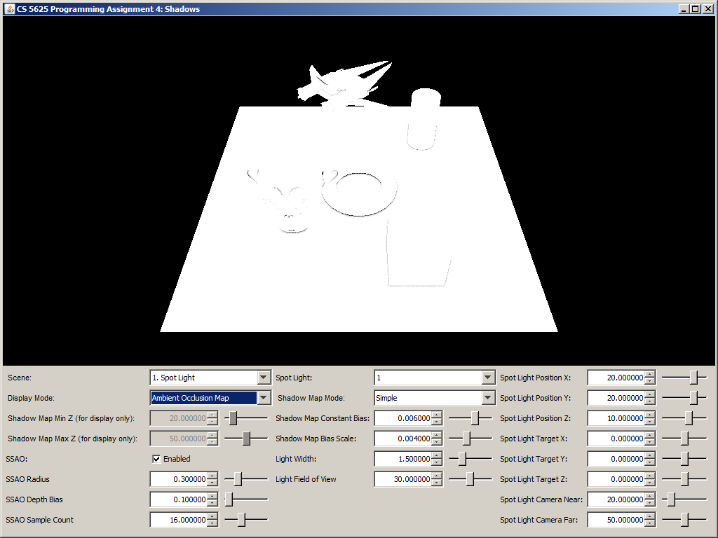
A correct implementation should yield the following results:
| Ambient Occlusion Buffer | Rendering with SSAO | Rendering without SSAO |
 |
 |
 |
 |
 |
 |
 |
 |
 |