CS5625 PA3 Sampling and Filtering

Out: Sunday March 15, 2015

Due: Friday March 27, 2015 at 11:59pm

Work in groups of 2.

Overview

In this programming assignment, you will implement:

antialiased sampling of a procedural test pattern,
high quality reconstruction for scaling of images, and
high quality anisotropic texture filtering,

all predominantly in GLSL fragment shaders. Some of them replicate features already present in the hardware, but since you implement them you will see how they work.

A few notes on the framework for this assignment:

There are three applications in the cs5625.pa3 package, one for each of the three tasks. Each displays a bare-bones UI with just the OpenGL viewport, and an appropriate set of mouse controls to move the images around and explore the aliasing artifacts that result. In the Supersample and Texfilter applications, the view deliberately lags behind the mouse, catching up exponentially so that you get slow movement that highlights Moiré patterns.
Each application makes an attempt to measure its performance and displays three numbers in the corner of the viewport: the duration of time taken to draw the frame, the interval between frames, and the frame rate, which is the reciprocal of the frame interval. These numbers are helpful in understanding how fast your program is running, but they need to be taken with a grain of salt because the Java windowing system takes up a lot of time, especially for large window sizes.
In order to measure performance, the applications render continuously, which means they will attempt to use all available CPU time. This can be annoying, and if you want a better behaved application when you are not worrying about framerate, you can modify the relevant GLView implementation for your platform, modifying it to use FPSAnimator at 30 or 60 frames per second rather than using the simple Animator class that redraws continuously.

Task 1: Sampling

In this task your job is to implement high-quality antialiased sampling of an analytically defined image. The image is a test pattern, known as a "zone plate" because of its resemblance to a diffractive optical element of the same name but actually a very simple function: $f_\text{zp}(x, y) = f_\text{sw}\bigg(\frac{x^2 + y^2}{s^2}\bigg)$ where $f_\text{sw}$ is a square wave: $f_\text{sw}(t) = \begin{cases} 0, & t - \lfloor t \rfloor < 0.5 \\ 1, & t - \lfloor t \rfloor >= 0.5 \end{cases}$ The fragment shader that should contain all the implementation for this task is zoneplate.frag.

Point sampling

The first part of this task is to implement this function in a fragment shader, simply evaluating it at the center of each pixel to produce a point-sampled, and highly aliased, result, similar to this image:

You'll want to set $s$ to a good value for your typical window size, so that you can see the broad circles near the origin but also see far enough away to see the patterns that happen near the Nyquist frequency and near the sample frequency. We used $s=50$ pixels but feel free to modify based on screen resolution.

The framework contains the code to draw a full-screen quad with the zoneplate.frag fragment shader, and it passes in a 2D point (controlled by mouse motion) where the center of the pattern should go, and an integer mode, controlled by key presses, that indicates what kind of sampling should be done. MODE_POINT is the default mode that corresponds to this subtask.

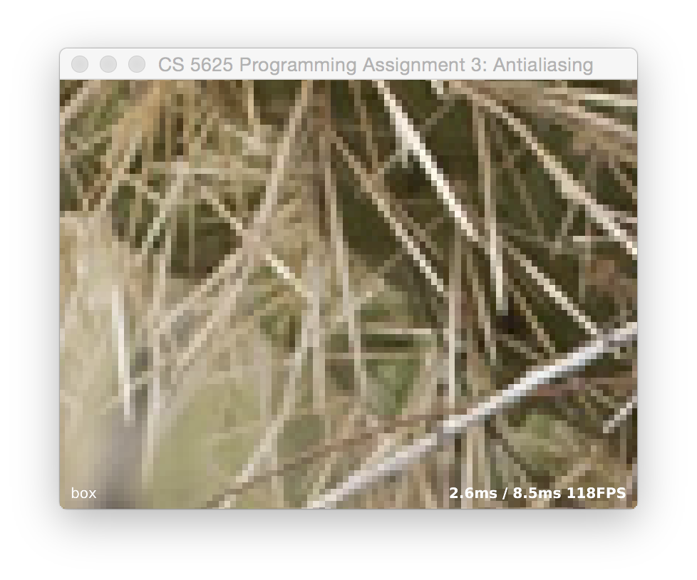
Box filtering

Once you have point sampling up and running, modify your shader so that when mode is MODE_BOX, for each pixel it averages $N^2$ samples of the same function, positioned in a $N\times N$ grid spread over a unit square (in pixel coordinates) centered at the pixel's sample position. (You can control $N$ using the + and - keys.) Once this is working, you should find that the jaggies on the circles near the center become smooth, and the Moiré patterns are greatly diminshed once $N$ gets to 4 or so, something like this:

(When you're looking at these images, note that your web browser may be layering its own resampling artifacts on top of the ones in the image; open the linked image in its own window to see it more clearly.)

If everything is working right, you should not see the pattern shift as you change $N$ ; the position of the main bull's-eye should remain the same while the edges get smoother.

Questions to ponder:

Watch the artifacts produced by the box filter. Why do some artifacts move around when you change the number of samples, but some stay put?
Which supersampling rates are good at eliminating the artifacts that happen at multiples of the sample frequency?
What happens in the frequency domain when we approximate a box filter with a grid of samples?
If you unroll the loop for a fixed value of $N$ does your shader run faster than the general one with for loops?

Gaussian weighted supersampling

With box filtering, things get better with increasing $N$ , up to a point, but many of the artifacts are persistent no matter how large we make $N$ . We can improve matters by weighting the samples with a smooth filter, though at the expense of needing to consider samples over a larger area.

Add the ability to compute a Gaussian filtered image with the same supersampling grid when mode is set to MODE_GAUSS. That is, when $N$ is 5, you should sample the function at 5 samples per pixel along each axis, and weight the results by a Gaussian filter. This means you will need to consider more samples for the same value of $N$ , because the support of the filter is wider.

Use a Gaussian with a standard deviation of 0.5 pixels—generally a good compromise between blurring and aliasing—and compute samples out to three standard deviations from the center. This means you will consider all the points on the supersampling grid that fall within a 3x3 box centered at the pixel center. You should find that the result has artifacts in roughly the same positions as the box filtered result for the same $N$ , but that the patterns are further reduced in contrast:

Experiment with reducing the limit of the filter's box; what kind of artifacts result from setting this too low? How about the standard deviation?

Poisson-disc sampling

To break up these spatially coherent patterns, we can use randomly positioned samples instead of the regular grid. A good way to do this is using Poisson disc patterns, which are sets of randomly positioned points arranged so as to maximize the minimum distance between points. You can find a Poisson disc patterns with 40 points over the unit square in this file. Further extend your fragment shader so that when mode is MODE_POISSON, it takes samples at positions defined by these points instead of on a regular grid.

You should find that the regular aliasing patterns become less grid-aligned, but are not much different in magnitude than the Gaussian filter for a comparable number of samples (that is, about N = 2 if you are going out to 3 standard deviations). This is because the sampling pattern is still a repeating pattern at the pixel frequency, since we are using the same pattern every time.

The right solution would be to have a different Poisson disc pattern for each pixel, but since the patterns need to be precomputed, this is not feasible. A standard trick is to randomly choose among several different patterns, or to rotate the pattern by a random angle at each pixel. Implement the rotation approach, for the case where mode is MODE_ROTPOISSON. To get pseudorandom numbers in a fragment shader, we can compute a hash function on the pixel coordinate: it will be different per pixel in a way that appears random. A hash function known to work well is here.

When you have this working, you should find that the grid-related artifacts are gone and replaced by random noise; the grid-independent artifacts are real, and they will still be there:

You can experiment with other sampling filters, such as Lanczos and other windowed-sinc functions, to see if you can quash these further without losing the detail in the image.

The Test Application

The test program for this task is implemented in the PA3_Supersample class. You can switch between sampling modes by pressing the following keys:

p: point sampling
b: box filtering
g: Gaussian weighted supersampling
d: Poisson disc sampling
r: rotated Poisson disc sampling

Also, as noted above, the number of samples

$N$ can be controlled by the + and - keys.

Task 2: Reconstruction

For the second task, you'll implement several reconstruction filters for enlarging an image in the upsample.frag. The test application for this part, PA3_Upsample, reads in an image and then provides it as a texture to a fragment shader running on a full-screen quad. The texture coordinates are set up to sample from a rectangle in the image—initially, the full image, but you can use the scroll wheel to zoom in and you can click and drag to move the image around on the screen.

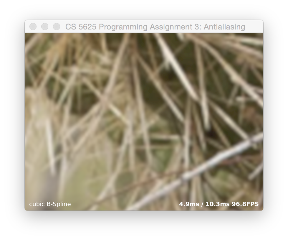
There are three filters to implement: box, tent, and cubic. Like the previous task, there is a keyboard-adjustable mode parameter that controls which filter is used. (The keys are listed at the end of this task.) The box corresponds to nearest-neighbor sampling, which happens by itself anyway. The tent corresponds to linear interpolation, similar to what we implemented during lecture. The cubic is a piecewise cubic function with radius of support 2, as described in the SIGGRAPH paper:

D. Mitchell & A. Netravali, “Reconstruction filters in computer graphics,” SIGGRAPH 1988.

in Equation 8. Mitchell and Netravali describe a family of cubics with two parameters,

$B$ and

$C$ , and recommend the values

$B = C = 1/3$ for general use. Set things up so that it uses those values for MODE_CUBIC_MN;

$B = 1, C = 0$ for MODE_CUBIC_BSP; and

$B = 0, C = 0.5$ for MODE_CUBIC_CR. The edges of the cactus spikes are quite sharp and need a pretty soft reconstruction to completely eliminate grid artifacts.

A correct implementation looks something like this:

If you have your indexing conventions consistent, the image should not shift around when switching between filters.

Mode Keys

b: MODE_BOX
t: MODE_TENT
c: MODE_CUBIC_CR
s: MODE_CUBIC_BSP
m: MODE_CUBIC_BSP

Task 3: Texture antialiasing

The final task combines the two previous tasks to deal with the thorny problem of texture filtering. Classic references on this topic include the following papers:

L. Williams, “Pyramidal Parametrics,” SIGGRAPH 1983.

N. Greene & P. Heckbert, “Creating Raster Omnimax Images from Multiple Perspective Views Using the Elliptical Weighted Average Filter,” Computer Graphics & Applications 6:6 (1986).

The fragment shader that should contain the implementation for the sampling operations in this task is texfilter.frag. The test application is implemented by the PA3_Texfilter class that uses the associated renderer TexfilterRenderer.

Nearest-neighbor sampling

The first part of this task is fairly simple: when mode is MODE_BOX, perform nearest-neighbor sampling. Because the rectangle texture we are using doesn't support the GL_REPEAT wrapping mode, you'll have to wrap the coordinates yourself, as well as scaling them to texel coordinates. (Q: how does the performance differ if you do this using if statements vs. doing it using floating point functions?)

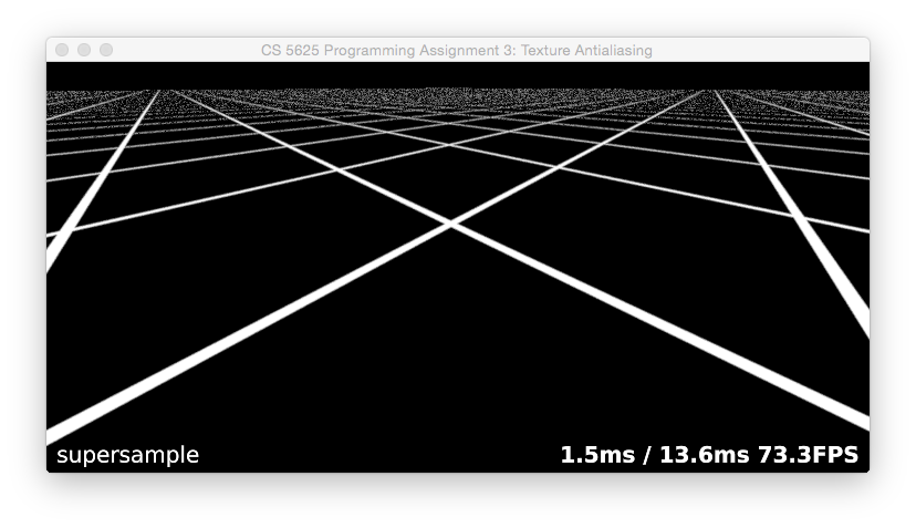
When you have this working, you should see a brick surface stretching to the horizon, and you should have a terrible mess of glittering, swimming Moiré patterns in the distance. To see even more dramatic results, switch to the texture grid2.png:

Supersampling

The simplest way to solve this problem is to average mutliple samples of the texture. You can do this in exactly the same way as you did supersampling for Task 1. Use the Poisson disc pattern to take 40 samples from the texture and average them with Gaussian weights. Since we want the samples to cover an area corresponding to the filter radius in image space, to find their positions in texture coordinates you will want to map them through the derivative matrix for the screen-to-texture mapping, which you can compute using the dFdx and dFdy builtins in GLSL.

When you have this working, you should find that it antialiases very well, though it runs a little slow and introduces a bit of shimmering noise:

Mipmapping

The standard, fast approach to texture filtering is to use mipmaps. Implementing a mipmap involves two parts: computing the images in the mipmap hierarchy, and sampling from the in a shader.

Building the mipmap. In order to keep control of the whole process in our shader where we can see it, we will build the mipmaps ourselves and put them into a single-layer texture, rather than using the mipmap data structures provided by OpenGL.

The plan is to precompute all the levels of a mipmap, and store them in a single texture of size $2N \times N$ where $N$ is the size of the base texture. A recommended scheme is to store the mipmap level $l$ , which is of size $N/2^l$ , with its lower left corner at $(N/2^l, 0)$ . (Since mipmap code is much simpler for power-of-two sized images, we will let the base texture be square, with $N$ equal to the smallest power of two that is at least as large as both the width and height of the source texture.)

Since we have the required filtering operations already implemented in fragment shaders, we'll do the mipmap generation on the GPU. Start by implementing the buildPyramid method in TexfilterRenderer. The method should make use of upsample.frag program to resample the texture directly into each of the mipmap levels. To do this, use glViewport to select the square region where the mipmap level goes, and then draw a full screen quad to copy the full width and height of the source texture into that viewport.

This will work well for the lowest (largest) levels of the pyramid, but will alias for the higher levels. We need filtering, but this can be done very efficiently by downsampling each level to form the next higher level. Implement this using the same upsampling shader, but modify it so that you can use it for downsampling, with the filter sized according to the resolution of the half-size output texture. You will need to write each level to a temporary buffer rather than writing directly into the mipmap buffer, because you can't read from the same texture you are writing to. A diagram may help:

Using the D key you can get the framework to show you this buffer. The result should look something like this, for the brick-256 texture:

Sampling from a single mipmap level. To complete this part, implement basic mipmapping. This means adding the MODE_TRILINEAR mode to your texture filtering shader, doing a linear interpolaton in the mipmap for each of two levels and blending them based on the desired level of detail. Start by using a single hardcoded level, to make sure you can successfully bilinearly interpolate from each of the mipmap levels. From left to right, level hardcoded to 0 and 2 for brick-256:

Note that this scene requires GL_REPEAT style texture wrapping: the texture coordinates on the plane run from 0.0 to 25.0 on each axis. But this mode is not supported for rectangle textures (and it wouldn't solve the problem anyway, since our tiles are smaller than the texture). Your shader will have to manually wrap the texture coordinates, or you will just get one copy of the brick texture, way off in a corner of the world.

Of course, for the brick-1024 texture, levels 2 and 4 would look similar.

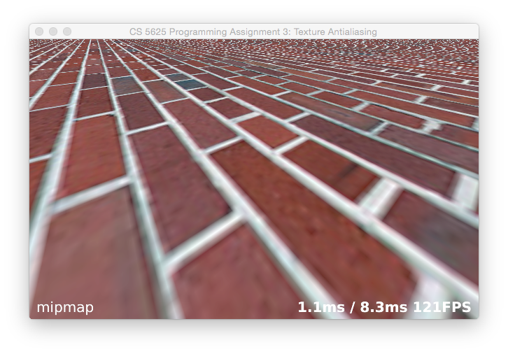
Sampling from the appropriate mipmap level. Once this works, compute the mipmap level using the same derivatives you used to implement the supersampling mode, using the formula recommended by Williams in the paper referenced above. Then you linearly interpolate between the integer levels on either side of the real-number mipmap level you compute. The result should look comparable to OpenGL's hardware mipmapping result (use the O key to flip back and forth):

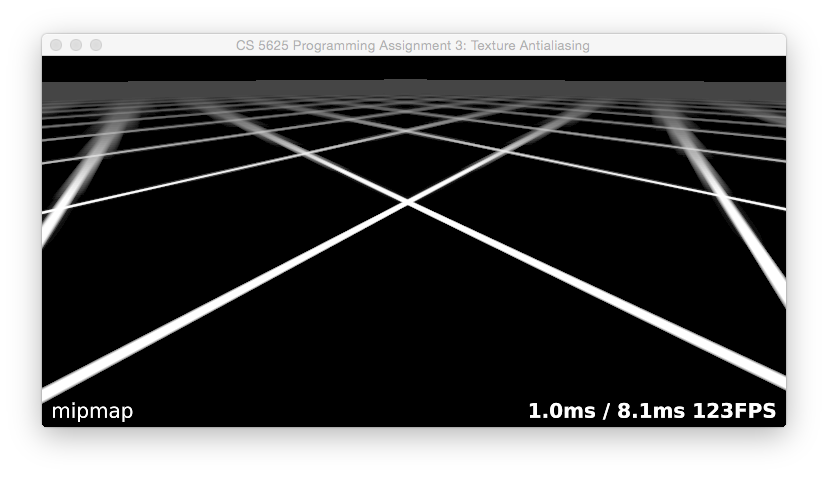
though the exact appearance of textures using the built-in mipmapping will differ slightly from system to system depending on the filters used to build the hierarchy.

Details, details, … Your images will not yet look quite like this; you'll notice there are some artifacts along the seams between tiles. Why? How can you fix them without killing performance? Go ahead and fix them so there are no major seams (though a discontinuity is OK—but it's simple enough to remove that also). Hint: in my implementation, the mipmap buffer for a 256 by 256 texture is 530 by 256, and this version is what's shown in the image above.

Anisotropic mipmapping

In this last section we will implement an anisotropic filtering method described in the following paper:

J. McCormack, R. Perry, K. Farkas, and N. Jouppi, “Feline: Fast Elliptical Lines for Anisotropic Texture Mapping,” SIGGRAPH 1999.

The main idea here is to average several lookups computed using your trilinear mipmapping code, with the lookup points positioned along the major axis of the ellipse defined by the texture coordinate derivatives.

Implementing anisotropic filtering is fairly simple given the working mipmap implementation. From the formulas in the paper, using the derivatives given to you by dFdx and dFdy, compute the minor and major axis length and the major axis direction. Select the mipmap level using the minor axis length, and make five lookups distributed along the major axis. Average them using Gaussian weights. That's it!

For those interested in the math behind the formulas, David Eberly's explanation from his Geometric Tools series is excellent:

D. Eberly, “Information About Ellipses,” geometrictools.com.

Mode Keys

b: nearest-neighbor sampling
s: supersampling
m: mipmap with trilinear interpolation
a: mipmap with anisotropic filtering
d: displaying the mipmap you computed
o: turning on OpenGL (only work with nearest-neighbor sampling and trilinear interpolation).

For this task it is instructive to look at the results of more than one texture; you can switch textures by editing the filenames that are hardcoded into the calls to the Texture*Data constructors in TexfilterRenderer.