CS5625 PA1 Shading Models and Techniques

Out: Thursday February 5, 2015

Due: Thursday February 19, 2015 at 11:59pm

Work in groups of 2.

Overview

In this programming assignment, you will implement a number of BRDF models to be used with two shading techniques: "forward" and "deferred" shading. You will also implement an algorithm to compute per-vertex tangent vectors of triangle meshes.

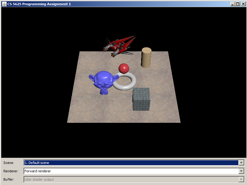
The PA1/student folder contains an Eclipse project that contains all the relevant source code. The class cs5625.pa1.PA1 implements a program that loads and renders three 3D scenes using 2 different renderers corresponding to the two mentioned rendering styles. Running the program, you should see the following window:

You can use the combo boxes at the bottom of the window to change the scenes and the renderers. For the "deferred" renderer, you have the option of selecting which buffer among five to display on the screen. We hope this feature will be useful for you when debugging your shaders. The program can be controlled using the following mouse and keyboard combinations:

• LMB or Shift+LMB: Rotating the camera.
• Alt+LMB: Translating the camera view point.
• Ctrl+LMB or Mouse Wheel: Changing the camera zoom.

Task 1: Blinn-Phong Shading Model in the Forward Renderer

In 4620, all real-time assignments used a rendering technique known as “forward” shading, where the lighting and shading of each fragment is computed immediately once the fragment is rasterized from the geometry. Forward shading is implemented in the class cs5625.pa1.ForwardRenderer. However, we have only provided implemented two types of materials: the "single color" material and the Lambertian one. In this task, we ask you to edit:

• PA1/student/src/cs5625/pa1/ForwardRenderer.java
• PA1/student/src/shaders/forward/blinnphong.frag

so that the renderer can handle the Blinn-Phong material as well. The Blinn-Phong material itself is implemented by the cs5625.gfx.material.BlinnPhongMaterial class, which you can inspect to see what fields and methods it has. However, you do not need to edit the class itself.

After finishing the implementation, the rendering of the default scene should look like the following:

Task 2: Isotropic Microfacet Shading Model

Edit

• PA1/student/src/cs5625/pa1/ForwardRenderer.java
• PA1/student/src/shaders/forward/isotropic_microfacet.frag

to implement the microfacet reflectance model describe in the paper "Microfacet Models for Refraction through Rough Surfaces" by Walter et al., using the GGX model for the normal distribution function (NDF) that was introduced (to graphics) by that paper. (Despite the name, the paper talks about models for both refraction and reflection. However, we will only use the reflection part.)

The parameters of the model are strored in the IsotropicMicrofacetMaterial class, and they are:

• The diffuse color $k_d$ in RGBA format.
• The index of refraction $\eta$, a scalar.
• The roughness parameter $\alpha$, a scalar.

The solution implemented the model as follows. The RGB color of the fragment due to a light source is given by: $$\mathrm{color} = \bigg( k_d + \frac{ F(\mathrm{i}, \mathrm{m}) D(\mathrm{m}) G(\mathrm{i}, \mathrm{o}, \mathrm{m})}{4 | \mathrm{i} \cdot \mathrm{n} | |\mathrm{o} \cdot \mathrm{n} | } \bigg) \max( 0, \mathrm{n} \cdot \mathrm{i} ) \times I$$ where

• $\mathrm{n}$ is the normal vector at the point being shaded,
• $\mathrm{i}$ is the unit vector from the shaded point to the light source,
• $\mathrm{o}$ is the unit vector from the shaded point to the camera,
• $\mathrm{m}$ is half vector between $\mathrm{i}$ and $\mathrm{o}$, in other words, $$\mathrm{m} = \frac{\mathrm{i} + \mathrm{o}}{\| \mathrm{i} + \mathrm{o} \|},$$
• $F(\mathrm{i}, \mathrm{m})$ is the Fresnel factor: $$F(\mathrm{i}, \mathrm{m}) = \frac{1}{2} \frac{(g-c)^2}{(g+c)^2} \bigg( 1 + \frac{(c(g+c)-1)^2}{(c(g-c)+1)^2} \bigg)$$ where $g = \sqrt{\eta^2 - 1 + c^2}$ and $c = |\mathrm{i} \cdot \mathrm{m}|$,
• $D(\mathrm{m})$ is the GGX distribution function: $$D(\mathrm{m}) = \frac{\alpha^2 \chi^+ (\mathrm{m} \cdot \mathrm{n})}{\pi \cos^4 \theta_m (\alpha^2 + \tan^2 \theta_m)^2}$$ where $\chi^+$ is the positive characteristic function ($\chi^+(a) = 1$ if $a> 0$ and $\chi^+(a) = 0$ if $a \leq 0$), and $\theta_m$ is the angle between $\mathrm{m}$ and $\mathrm{n}$,
• $G(\mathrm{i}, \mathrm{o}, \mathrm{m})$ is the shadowing-masking function of the GGX distribution: $$G(\mathrm{i}, \mathrm{o}, \mathrm{m}) = G_1(\mathrm{i},\mathrm{m}) G_1(\mathrm{o}, \mathrm{m})$$ and $$G_1(\mathrm{v},\mathrm{m}) = \chi^+((\mathrm{v} \cdot \mathrm{m}) (\mathrm{v} \cdot \mathrm{n})) \frac{2}{1 + \sqrt{1 + \alpha^2 \tan^2 \theta_v}}$$ where $\theta_v$ is the angle between $\mathrm{v}$ and $\mathrm{n}$.
• $I$ is the "power" of the light source. See more details on how the power is computed in the implementation details section.

Task 3: Tangent space computation

When shading with an anisotropic model or computing normals from a tangent-space normal map (which will be covered in the next PA), a complete orthogonal coordinate system at the shaded point is needed. This means we need to define two orthogonal vectors perpendicular to the surface normal at each point on the surface—these vectors span the tangent space to the surface at that point, and together with the normal vector, $\mathrm{n}$, they are often called the tangent frame.

It's important to have a consistent way to choose these tangent vectors, and the usual way is to define them based on the texture coordinates. Let the first tangent vector, $\mathrm{t}$, called just the “tangent,” point in the direction that the first texture coordinate, $u$, increases (so that it's tangent to the lines of constant $v$), and let the second tangent vector, $\mathrm{b}$, called the “bitangent,” complete a right-handed orthonormal basis.

In this task, edit the computeTangents method of the TriMesh class to compute the tangent space at each vertex of a triangle mesh according to the algorithm given in this web page. Be sure to appropriately cite this source in your code.

Task 4: Anisotropic Microfacet Shading Model

With the tangent space computed, you are now ready to implement the anisotropic version of the microfacet shading model. For an anisotropic surface, the NDF is no longer a function only of the angle between the normal and the half vector, but depends on the components of the half vector in the $\mathrm{t}$ and $\mathrm{b}$ directions independently. The model we'll use is almost the same as the isotropic one. The only differences are in $D$ and $G_1$, which must now be calculated using the tangent space and two roughness parameters $\alpha_X$ and $\alpha_Y$, specificed separately to indicate the width of the NDF in the direction of $\mathrm{t}$ and $\mathrm{b}$ respectively.

Consider the coordinate frame with the tangent $\mathrm{t}$ as its x-axis, the bitangent $\mathrm{b}$ as its y-axis, and the surface normal $\mathrm{n}$ as its z-axis. Let $m_t$, $m_b$, and $m_n$ be the scalars such that $$\mathrm{m} = m_t \mathrm{t} + m_b \mathrm{b} + m_n \mathrm{n}.$$ (Note that $m_n = \mathrm{m} \cdot \mathrm{n} = \cos \theta_m$, $m_t = \mathrm{m} \cdot \mathrm{t}$, and $m_b = \mathrm{m} \cdot \mathrm{b}$.) Then, the anisotropic version of the GGX distribution is given by: $$D(\mathrm{m}) = \frac{\chi^+(\mathrm{m} \cdot \mathrm{n})}{ \pi \alpha_X \alpha_Y \bigg(m_n^2 + \frac{m_t^2}{\alpha_X^2} + \frac{m_b^2}{\alpha_Y^2} \bigg)^2}.$$ (See if you can show that the above expression is the same as the definition of $D$ in Task 2 when $\alpha_X = \alpha_Y$.) The shadow masking function $G$ is the same as that of the isotropic function, except that the roughness parameter $\alpha$ must be calculated from $\alpha_X$ and $\alpha_Y$ as follows: $$\alpha = \sqrt{\frac{\alpha_X^2 m_t^2 + \alpha_Y^2 m_b^2}{m_t^2 + m_b^2} }.$$

Edit

• PA1/student/src/cs5625/pa1/ForwardRenderer.java
• PA1/student/src/shaders/forward/anisotropic_microfacet.frag

to put the above formulas into action. After completing this exercise, the rendering of the "material test" scene (3rd scene in the combo box) should look like the image below.

From another view points:

Task 5: Deferred Shading

We have been implementing forward shading in the last 4 tasks. Nevertheless, forward shading has one main drawback: if the scene has many overlapping objects, expensive lighting calculations are performed for all fragments, even those that will be overwritten by an object closer to the viewer. Deferred shading addresses the shortcoming as follows:

1. Instead of lighting each fragment as it is generated, the scene is first rendered into an off- screen buffer (the “g-buffer”) using simple shaders which just output material properties. Since no lighting or other computation has been done yet, overlapping objects are handled efficiently.
2. Run an “übershader” on the g-buffer to compute shading. This shader is usually called an "übershader" ("supershader") since it contains lighting code for all types of lights and materials.

However, deferred shading cannot handle transparency or translucency. Since we will have some of them in later assignments, we will keep the option open by implementing both rendering techniques.

The class cs5625.pa1.DeferredRenderer implements the deferred shading technique. It makes uses of the shaders located in the student/src/shaders/deferred directory. You will see that the directory contains vertices and fragments shaders for the five materials we have implemented for the forward renderer. However, only the "single color" material has been implemented, and it's your job to port the rest of the materials to the deferred shading world. This also involves editing the übershader so that it knows how to deal with other types of materials.

As mentioned earlier, the shaders for each material will not compute the final fragment color, but will fill the g-buffers with information useful for computing it later. Depending on the material, this information includes the position of the fragment, the normal vector, the tangent vector, the diffuse and specular color, the ID of the material, and other material-specific parameters. DeferredRenderer uses 4 g-buffers each of whose pixels can store 4 floating points numbers, totalling 16 floating point numbers. The provided implementation of the single color material also requires that the first floating point number of the first g-buffer stores the material ID. As a result, you have 15 floating points numbers to encode all other information. We leave this encoding up to you.

The übershader should figure out the material being shaded from the material ID and then compute the final fragment color accordingly. Since you have implemented all the materials in the forward renderer, implementing the übershader should be as simple as copying and pasting the relevant code from the forward shaders (with appropriate modifications, of course).

You should check the correctness of your deferred renderer by comparing its output to that of the forward renderer. All renderings they generate should be the same.

Hardware Requirements

The framework for the programming assignements not run on older (or netbook) hardware. Known requirements are:

1. The GPU must support OpenGL 2.0 and GLSL 1.2.
2. The GPU must support the GL_ARB_texture_rectangle extension.
3. The GPU must support at least 4 color attachments on a frame buffer object.
4. The GPU must support at least 5 texture targets.
5. The GPU must suport dynamic branches and loops in fragment shaders. On the GPU tested which didn't support this, it rendered black instead of the correct output from the übershader, and didn't generate any errors. If you see this problem and you absolutely can’t use a newer graphics card, you can try temporarily replacing the light_count uniform in the übershader with a constant. Remember to change it back (and test that it works) before submitting.

All Gates Hall lab computers have up-to-date GPUs and should be able to run the framework without problems.

What to Submit

You should submit a ZIP file containing all the source codes and data in the PA1/student directory. All the code you have written should be well commented and easy to read, and header comments for all modified files should appropriately indicate authorship. Be sure to cite sources for any code or formulas that came from anywhere other than your head or this assignment document. Also, put in the directory a readme file explaining any implementation choices you made or difficulties you encountered.

Implementation Details

Use of Textures

Some material properties are stored as a scalar/vector value and a texture. For example, in the BlinnPhongMaterial class, there is both the specularColor field and teh specularTexture field. In such a case, the scalar/vector value must be defined, but the texture can be left unspecified (i.e., null).

In the corresponding fragment shader, there will be 3 uniforms related to the material parameter. One uniform corresponds to the scalar/vector value (for example, mat_specular). One uniform serves as a flag telling whether there exists the corresponding texture (for example, mat_hasSpecularTexture). One uniform corresponds to the texture (for example, mat_specularTexture). If the texture is undefined, you should use the scalar/vector value to calculate shading. If the texture is undefined, you should fetch the texture value, multiply it with the scalar/vector value, and use the product to compute shading. For example, we might compute the specular value that will used later for shading in the fragment shader as follows:

vec3 specular = mat_specular;
if (mat_hasSpecularTexture) {
  specular *= texture2D(mat_specularTexture, geom_texCoord).xyz;
}

Point Light Sources

Light sources in this PA are all point light sources and implemented in the PointLight class. A point light is specified by three parameters: its position, its color (i.e., power), and its 3 attenuation coefficients. The power reaching a shaded point is computed in a non-physical manner as follows: $$\mathrm{power} = \frac{color}{A + Bd + Cd^2}$$

where $d$ is the distance between the light source and the shaded point, $A$ is the constant attenuation coefficient, $B$ is the linear attenuation coefficient, and $C$ is the quadratic attenuation coefficient. You can see this calculation implemented in the fragment shader of the lambertian material.