Lecture notes by Tom Roeder
In the last lecture, we discussed an information flow policy called Noninterference. Our discussion of it led to a rather conservative set of rules: any low output that is at all dependent on a high secrecy variable is regarded as giving away information about that high variable. Clearly there are functions that give away very little information about some of their inputs. For example, encryption, by design, gives away almost no information at all. In general, we would like to be able to characterize the amount of information that is leaked from a given operation, and have our characterization be more precise than just "leak" or "no leak". We want a quantitative measure of information flow. We can measure this sort of quantitative information flow using tools from Information Theory.
Let's recall some definitions from information theory. Those who desire more in-depth discussion of these definitions and results should look at any introductory information theory text. In this lecture we use common terms that are well discussed in the literature.
Let's start by giving a definition of the core concept: information. Information is the enemy of uncertainty. You have acquired information about a topic if you become more certain about it (hopefully, for instance, you are less uncertain about security now than when you started taking CS513). Similarly, you can imagine the state of your uncertainty while playing cards. At the beginning of a game, no cards have been exposed, and (hopefully) you don't know where any of the cards are in the deck. Thus you have uncertainty about the order of the cards. As soon as you are dealt one, however, you have gained information and reduced your uncertainty: now you know one of the cards. The two principal ideas we will use to describe this reduction in uncertainty are entropy and equivocation. Information theory measures uncertainty with entropy.
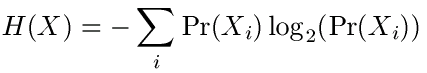
We can define entropy as follows: suppose that you have a system that can send n distinct messages. We will write them as X1, ..., Xn. Each of these messages is sent with a given probability pi = Pr(Xi). (of course, we have that 0 ≤ pi ≤ 1 and åi pi = 1. Those who have taken probability will recognize X as a random variable.) Entropy is then a measure of how uncertain it is which message will actually be sent. We define the entropy of the system X as
We have already said that one way to think about entropy is a definition of uncertainty. In particular, we can say that the entropy of a message is the average amount of information in bits that message contains. Let's look at an example to see how this works in practice. Consider a fair coin C. In this situation, the "messages" are Heads and Tails, and since the coin is fair, each message has probability 1/2. What is the entropy?
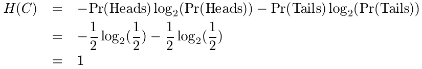
Thus each flip of the coin contains 1 bit of information. You can also view this result in another way: the optimal encoding of a coin flip takes up exactly 1 bit. This is intuitive if you think about it: there are only two possible results from the coin flip, and 1 bit has two states with which it can represent these results. What would be the result if we had a double headed coin? As a check that you understand, see if you can verify that H = 0 in this case. Since the coin will always come up heads, we need no bits to represent the results.
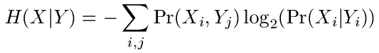
Now we can define equivocation as conditional entropy; equivocation is the amount of uncertainty you have about a given message if you know that some other message has already occurred. This concept is closely related to the concepts of joint and conditional probabilities. Given any two systems X and Y, we can define
Equivocation is defined as:
Given these definitions, we can show that we will always have H(X) ≥ H(X | Y), that is, conditioning (gaining information) can never increase uncertainty. To understand equivocation, we can think again about playing cards. Suppose that no cards have been turned over. What is your uncertainty about what the first card will be? It could be anything, so you have no information. If now we assume that the first card is turned up and it is the Ace of Hearts, what is your uncertainty about what the second card can be? It is less than the first time, since you know it can't be the Ace of Hearts.
We can also consider equivocation in the context of variables. Suppose that x is a 32-bit variable drawn from a uniform distribution (entropy is maximized in a uniform distribution). It is clear that in this case, H(X) is 32 bits, since we have no information about the value of this variable. What happens if we learn the parity of the variable? Since the parity gives us one bit of information, we now know that H(X|parity(X)) = 31 bits.
Given these definitions, we can now work out examples in which we can see the exact number of bits that are flowing from one variable to another. We will use the following notation: S is a program. x and y are variables, and X and Y are systems for x and y. Y' is the system for y after execution of S.
For example, we might have the following scenario: x is an integer in [0, 15] with a uniform distribution. X has messages X0, ..., X15 and Pr(Xi) = 1/16.
Given a program S, we can figure out what the flow is from x to y by calculating the reduction in uncertainty between the states of the systems before execution of S and that after. We represent these uncertainties as the equivocation of X given Y and Y', respectively. This comes out as a formula for the leakage L in S from x to y.
![]()
We might wonder why we don't simply compute the entropy of X for the initial uncertainty. In our computation, we consider X as secret information, and Y as public. Thus Y is given, since as public information, it is known to everyone. This equation then measures the difference between the initial and final uncertainties about X. We can do the following example to see how this works.
Suppose that x is in [0,15] uniformly distributed, y is certainly 0, and S = "y := x". We need to figure out the probabilities that occur in our formula: Pr(x = i, y = j), Pr(x = i | y = j), Pr(x = i, y' = j) and Pr(x = i | y' = j).
Since we know that y = 0, the value of this probability anywhere y is not 0 will be 0. Since x uniformly takes on the values in [0, 15], its probability in the case y = 0 is 1/16. This leads to the result
if j = 0, then 1/16
else 0
Again here we know that y = 0, and so the value of this probability anywhere y is not 0 will be 0. Since x still uniformly takes on the values in [0, 15], its probability in the case y = 0 is still 1/16. This leads to the result
if j = 0, then 1/16
else 0
Since we are evaluating the expression "y := x", we know that only those probabilities where x = y will be non-zero. Since there are 16 such probabilities, and all of them are equally likely, this means that we have
if i = j, then 1/16
else 0
The value of this probability is slightly more subtle. Since we are given the value of y, we know that the probability of x being the same value is 1, since we are evaluating an assignment statement. Thus we have
if i = j, then 1
else 0
We can plug these values into our equation to discover how many bits leak from x to y.
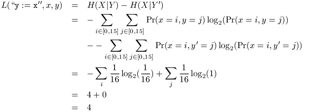
We should not be surprised to see that 4 bits leak from x to y. Since we are doing an assignment statement, all the bits of x should leak. Since we only need 4 bits to represent all the numbers from 0 to 15, this is exactly what is happening.
Jif is a Cornell CS project in Andrew Myers' group that adds information flow annotations and analysis to Java. The central idea in this system is to use a decentralized label model [Myers and Liskov 2000]. In this model, we do not use H or L as labels, but rather each label gives a set of policies owned by some principals. Conceptually, a policy has 1 owner, and makes statements about any number of readers. These policies are written Alice: Alice, Bob (or, in Jif, int {Alice: Alice, Bob} x;), which says that Alice owns this policy, and allows Alice and Bob to read the data with which this label is associated. To make any of this make sense, the owners and readers must be principals.
For a given label, it is possible to have more than one policy from
different principals applied at the same time. All policies in a
label are enforced. Suppose for instance that we had a policy that
had the following annotations: {Alice: Alice, Bob; Bob: Bob}.
Enforcing both policies here means taking the intersection of the
reader set; in our example, this means that only Bob can read
the data. In other words, a policy is said to be satisfied if at
most the readers specified in the policy can read the data.
Putting a reader in a policy is not a guarantee that they can read it.
It may even be the case that the intersection of two reader sets is
null, as in the example: {Alice: Alice; Bob: Bob}. In this
case, no principal can read the data, since we need to enforce both
policies.
Note that if a principal does not specify a policy in a label, then they
allow all readers to read the data. For example {Alice: Alice, Bob; Bob:
Bob} is a
label that does not mention Cindy, so Cindy implicitly allows any
principal to read data with this label.
Let's work out the details of a realistic application to see how this works. Our application is a Web tax preparation service. Bob, the consumer, has tax data and does not want to prepare his own tax forms. Preparer is a principal that has proprietary data and algorithms that he uses to prepare tax returns for a consumer. We can see how it works in the following diagram.
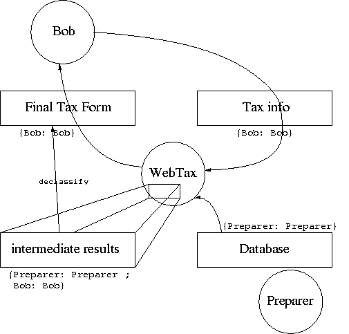
Since Bob wants the WebTax service to create a tax return for him to file, he must provide his tax data to it. He doesn't want to trust the Preparer with his information, however, so he adds a label: {Bob: Bob}. The Preparer is willing to use his proprietary data to prepare the tax return, but doesn't want Bob to have access to all his data (if he let Bob read all his data, Bob would have no need to pay for the Preparer's services). The Preparer thus adds a label to his data: {Preparer: Preparer}. The WebTax program is not a principal, just a program running on a machine. It can read the tax information from Bob and the data from the preparer, but label on the result is {Preparer: Preparer; Bob: Bob}, it can't actually release the results to anyone. (Note that the issue of whether or not the correct software is running in this instance is an orthogonal problem. We will simply assume for this example that WebTax is going to obey the policies in the labels.) Thus the Preparer must temporarily give authority to WebTax for the intermediate results to be declassified to {Bob: Bob}. Although the Preparer has an incentive to keep his data secret, we presume that he finds it in his best interest to give the completed tax forms to his paying customers. This leaks some information, but the Preparer gets paid for the leakage.
We saw in the above example that data sometimes is labeled such that principals cannot read it, but some external policy specifies that the labels should be relaxed so that they can. In this case, we need declassification. This operation creates a purposeful violation of noninterference. Presumably the principal that performs the declassification has some reason for being willing to change their policy. In the above example, it was because Bob had paid the preparer to do his taxes for him. Declassification always involves a downgrading of a security policy. Although in the tax example the Preparer's policy was entirely removed, declassification can be selective; a principal that owns a policy can remove particular elements from that policy. Thus, for example, Bob can change {Bob: Alice, Bob; Alice: Charlie} to {Bob: Alice; Alice: Charlie} or {Bob: Bob; Alice: Charlie}, but he cannot change it to {Bob: Alice, Bob; Alice: Charlie, Bob} or {Bob: Alice, Bob}. A principal can only modify policies they own.
Note that declassification is a dangerous operation! Afterwards, more principals can read the information than before. Because it is an explicit violation of noninterference, it is made explicit in the source code by a declassification statement. When we declassify, we must be sure that Bob has granted the code permission to be declassified. Thus we need some mechanism that will allow us to determine if the code has Bob's authority to do so. We might, for instance, check to see if Bob signed this code, and if so, to assume that it means that he gives it permission to declassify this data. Jif contains mechanisms for expressing and verifying such authority.
Recall from the first information flow lecture that we had some
notation for comparing labels. We used the symbol ![]() for this purpose. For
instance, we would write L
for this purpose. For
instance, we would write L ![]() H to say that L was less than H
in terms of secrecy. In this lecture, we will use the same symbol,
and will read it as "at most as restrictive as".
H to say that L was less than H
in terms of secrecy. In this lecture, we will use the same symbol,
and will read it as "at most as restrictive as".
Thus we can say that l1
![]() l2 when
l2 when
For example, {Bob: A, B} ![]() {Bob: A, B; Alice: A, B}
{Bob: A, B; Alice: A, B}
For example, {Alice: A, B} ![]() {Alice: A}
{Alice: A}
In our last lecture, we also had an operation that we could use to
combine two label sets. We wrote it ![]() . This operation took the least upper bound of two
labels, so, for instance, L
. This operation took the least upper bound of two
labels, so, for instance, L ![]() H = H. We can define such an operation
for these new labels as well. l1
H = H. We can define such an operation
for these new labels as well. l1 ![]() l2 is the least
restrictive policy such that
l2 is the least
restrictive policy such that
We need to think more carefully about what it means for a process to
be running with Bob's authority. Although it may have his authority,
he may not be the one running it. This is reminiscent of the
"speaks-for" relation that we discussed several lectures ago. The
process speaks for Bob: in Jif, this is called "acts for".
Principals are allowed to act for other principals. As in the speaks
for relation, we can get chains of acts-for relations between
principals. We also may have an individual that acts for a group.
For example, a lawyer acts for a client, and a boss acts for an
employee (assuming that the employee agrees to this relation). We can
then draw a hierarchy of principals and use the arrow A ![]() B to mean "A
acts for B". The following two diagrams are examples of what such
hierarchies might look like.
B to mean "A
acts for B". The following two diagrams are examples of what such
hierarchies might look like.
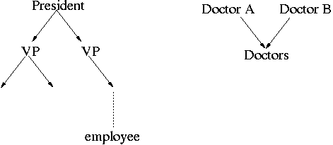
In the first example, the president acts for each of the vice-presidents, who in turn act for the members of their organization, and so on down the tree. Transitively, the president acts for the whole company. The opposite type of structure occurs when we have many individuals acting directly for a group (as opposed to a leader acting for the organization). The second example shows two doctors, each of which acts for the given group of doctors.
For more information about Jif, see http://www.cs.cornell.edu/jif.