Gradients
Many, if not most, machine learning training algorithms use gradients to optimize a function.
What is a gradient?
Suppose I have a function $f$ from $\R^d$ to $\R$. The gradient, $\nabla f$, is a function from $\R^d$ to $\R^d$ such that
$$\left(\nabla f(w) \right)_i = \frac{\partial}{\partial w_i} f(w) = \lim_{\delta \rightarrow 0} \frac{f(w + \delta e_i) - f(w)}{\delta},$$that is, it is the vector of partial derivatives of the function.
Another, perhaps cleaner (and basis-independent), definition is that $\nabla f(w)^T$ is the linear map such that for any $\Delta \in \R^d$
$$\nabla f(w)^T \Delta = \lim_{a \rightarrow 0} \frac{f(w + a \Delta) - f(w)}{a}.$$More informally, it is the unique vector $\nabla f(w_0)$ such that $f(w) \approx f(w_0) + (w - w_0)^T \nabla f(w_0)$ for $w$ nearby $w_0$.
Symbolic differentiation
Deriving gradients as we would do by hand is called symbolic differentiation.
- Write your function as a single mathematical expression.
- Apply the chain rule, product rule, et cetera to differentiate that expression.
- Execute the expression as code.
import sympy
x = sympy.symbols("x")
x
f = x*x + 4
f
f.diff()
Symbolic differentiation: Problems
The naive symbolic differentiation approach has a couple of problems.
- Converting code into a mathematical expression is not trivial! You'd need some sort of reflection capability.
- There's no guarantee that the computational structure of our original code will be preserved.
- Expressions you get from naive symbolic differentiation can be larger and more complicated than the thing we're differentiating.
f = sympy.sin(sympy.sin(sympy.sin(sympy.sin(sympy.sin(x)))))
f
f.diff()
An Illustrative Example
Imagine that we have some functions $f$, $g$, and $h$, and we are interested in computing the derivative of the function $f(g(h(x)))$ with respect to $x$. By the chain rule, $$ \frac{d}{dx} f(g(h(x))) = f'(g(h(x))) \cdot g'(h(x)) \cdot h'(x). $$ Imagine that we just copy-pasted this math into python. We'd get
def grad_fgh(x):
    return grad_f(g(h(x))) * grad_g(h(x)) * grad_h(x)
This code recomputes $h(x)$ twice!
To avoid this, we could imagine writing something like this instead:
def better_grad_fgh(x):
    hx = h(x)
    return grad_f(g(hx)) * grad_g(hx) * grad_h(x)
This code only computes $h(x)$ once. But we had to do some manual work to pull out common subexpressions, work that goes beyond what the plain chain rule gives us.
Now you might ask the very reasonable question: So what? We just recomputed one function. Could this really have a significant impact on performance?
To answer this question, suppose that we now have functions $f_1, f_2, \ldots, f_k$, and consider differentiating the more complicated function $f_k(f_{k-1}(\cdots f_2(f_1(x)) \cdots))$. The chain rule will give us \begin{align*} &\frac{d}{dx} f_k(f_{k-1}(\cdots f_2(f_1(x)) \cdots)) \\&\hspace{2em}= f_k'(f_{k-1}(\cdots f_2(f_1(x)) \cdots)) \cdot f_{k-1}'(f_{k-2}(\cdots f_2(f_1(x)) \cdots)) \\&\hspace{4em}\cdots f_2'(f_1(x)) \cdot f_1'(x). \end{align*} If each function $f_i$ or $f_i'$ takes $O(1)$ time to compute, how long can this derivative take to compute if
- ...I just copy-paste naively into python?
- ...I do something to save redundant computation?
Symbolic Differentiation: Take-away point
Computing a derivative by just applying the chain rule and then naively copying the expression into code can be asymptotically slower than other methods.
Numerical Differentiation
$$\nabla f(w)^T \Delta = \lim_{a \rightarrow 0} \frac{f(w + a \Delta) - f(w)}{a}.$$Therefore, for small $\epsilon > 0$,
$$\nabla f(w)^T \Delta \approx \frac{f(w + \epsilon \Delta) - f(w)}{\epsilon}.$$It's often better to use the symmetric difference quotient instead:
$$\nabla f(w)^T \Delta \approx \frac{f(w + \epsilon \Delta) - f(w - \epsilon \Delta)}{2 \epsilon}.$$Let's Test Numerical Differentiation
import math

def f(x):
    return 2*x*x*x-1

def dfdx(x):
    return 6*x*x

def numerical_derivative(f, x, eps = 1e-4):
    return (f(x+eps) - f(x-eps))/(2*eps)

print(dfdx(2.0))
print(numerical_derivative(f, 2.0, eps=1e-16))
24.0
0.0
Problems with Numerical Differentiation
- numerical imprecision (bigger problem as number of operations increases)
- if $f$ is not smooth, then wrong results
- unclear how to set $\epsilon$
- for a vector -> scalar function, you have to compute each partial individually, meaning $O(d)$ blowup in cost
- if you set $\epsilon$ too small, you can get zeros
Automatic Differentiation
Compute derivatives automatically without any overheads or loss of precision.
Two rough classes of methods:
- Forward mode
- Reverse mode
Forward Mode AD
- Fix one input variable $x$ over $\mathbb{R}$.
- At each step of the computation, as we're computing some value $y$, also compute $\frac{\partial y}{\partial x}$.
- We can do this with a dual numbers approach: each number $y$ is replaced with a pair $(y, \frac{\partial y}{\partial x})$.
Forward Mode AD Demo
import numpy as np

def to_dualnumber(x):
    if isinstance(x, DualNumber):
        return x
    elif isinstance(x, float):
        return DualNumber(x)
    elif isinstance(x, int):
        return DualNumber(float(x))
    else:
        raise Exception("couldn't convert {} to a dual number".format(x))

class DualNumber(object):
    def __init__(self, y, dydx=0.0):
        super().__init__()
        self.y = y
        self.dydx = dydx

    def __repr__(self):
        return "(y = {}, dydx = {})".format(self.y, self.dydx)

    # operator overloading
    def __add__(self, other):
        other = to_dualnumber(other)
        return DualNumber(self.y + other.y, self.dydx + other.dydx)
    def __sub__(self, other):
        other = to_dualnumber(other)
        return DualNumber(self.y - other.y, self.dydx - other.dydx)
    def __mul__(self, other):
        other = to_dualnumber(other)
        return DualNumber(self.y * other.y, self.dydx * other.y + self.y * other.dydx)
    def __pow__(self, other):
        other = to_dualnumber(other)
        return DualNumber(self.y ** other.y,
            self.dydx * other.y * self.y ** (other.y - 1) + other.dydx * (self.y ** other.y) * np.log(self.y))
    def __radd__(self, other):
        return to_dualnumber(other).__add__(self)
    def __rsub__(self, other):
        return to_dualnumber(other).__sub__(self)
    def __rmul__(self, other):
        return to_dualnumber(other).__mul__(self)

def exp(x):
    if isinstance(x, DualNumber):
        return DualNumber(np.exp(x.y), np.exp(x.y) * x.dydx)
    else:
        return np.exp(x)

def sin(x):
    if isinstance(x, DualNumber):
        return DualNumber(np.sin(x.y), -np.cos(x.y) * x.dydx)
    else:
        return np.sin(x)

def forward_mode_diff(f, x):
    x_dual = DualNumber(x, 1.0)
    return f(x_dual).dydx
print(dfdx(2.0))
print(numerical_derivative(f, 2.0))
print(forward_mode_diff(f, 2.0))
24.0
24.00000002002578
24.0
def g(x):
    return 12 + 4*x

print(numerical_derivative(g, 2.0))
print(forward_mode_diff(g, 2.0))

def h(x):
    return x**5.0

def dhdx(x):
    return 5*x**4

print(dhdx(2.0))
print(forward_mode_diff(h, 2.0))
3.9999999999906777
4.0
80.0
80.0
Problems with Forward Mode AD
- Differentiate with respect to one input
- If we are computing a gradient of $f: \mathbb{R}^d \rightarrow \mathbb{R}$, blow-up proportional to the dimension $d$
Forward Mode AD Takeaways
- Each operation in the original program is replaced with two operations
- one to compute the value $y$ (same as original)
- one to compute the derivative $\frac{\partial y}{\partial x}$
- The new operation has an analogous structure to the original one
- since its the derivative
- e.g. a matrix multiply would produce a new matrix multiply
- If the original operation had compute cost $C$, the new operation has cost $O(C)$.
Implementing Forward Mode AD
In Python, we can use operator overloading and dynamic typing. Suppose I write a function
def f(x):
    return x*x + 1.0
imagining that we will call it with x being a floating-point number.
- I can still call it with
xbeing a dual number (because Python is not explicitly typed). - When I do this, the operators
*and+desugar to calls to my__mul__and__add__methods. - I can do the differentiation in these methods.
- I can do this across the whole program to differentiate compositions of functions!
Benefits of Forward Mode AD
- Simple in-place operations
- Easy to extend to compute higher-order derivatives
- Only constant factor increase in memory use, since each $\frac{\partial y}{\partial x}$ object is the same size as $y$ and is only live when $y$ is
Problems with Forward Mode AD
- Differentiate with respect to one input
- problematic for ML, where we usually want to compute gradients
- If we are computing a gradient of $f: \mathbb{R}^d \rightarrow \mathbb{R}$, blow-up proportional to the dimension $d$
Reverse-Mode AD
- Fix one output $\ell$ over $\mathbb{R}$
- Compute partial derivatives $\frac{\partial \ell}{\partial y}$ for each value $y$
- Need to do this by going backward through the computation
Problem: can't just compute derivatives as-we-go like with forward mode AD.
Backpropagation: The usual type of Reverse-AD we use
Same as before: we replace each number/array $y$ with a pair, except this time the pair is not $(y, \frac{\partial y}{\partial x})$ but instead $(y, \nabla_y \ell)$ where $\ell$ is one fixed output.
- I use $\ell$ here because usually in ML the output is a loss.
- Observe that $\nabla_y \ell$ always has the same shape as $y$.
Deriving Backprop from the Chain Rule
Suppose that the output $\ell$ can be written as $$\ell = f(u), \; u = g(y).$$ Here, $g$ represents the immediate next operation that consumes the intermediate value $y$ (producing a new intermediate $u$), and $f$ represents all the rest of the computation. Suppose all these expressions are scalars. By the chain rule, $$\frac{\partial \ell}{\partial y} = g'(y) \cdot \frac{\partial \ell}{\partial u}.$$ That is, we can compute $\frac{\partial \ell}{\partial y}$ using only "local" information (information that's available in the program around where $y$ is computed and used) and $\frac{\partial \ell}{\partial u}$.
Deriving Backprop from the Chain Rule
More generally, suppose that the output $\ell$ can be written as $$\ell = F(u_1, u_2, \ldots, u_k), \; u_i = g_i(y).$$ Here, the $g_1, g_2, \ldots, g_k$ represent the immediate next operations that consume the intermediate value $y$ (note that there may be many such $g$), the $u_i$ are the arrays output by those operations, and $F$ represents all the rest of the computation. By the multivariate chain rule, $$\nabla_y \ell = \sum_{i=1}^k D g_i(y)^T \nabla_{u_i} \ell.$$ Again, we see that we can compute $\frac{\partial \ell}{\partial y}$ using only "local" information and the gradients of the loss with respect to each array that immediately depends on $y$, i.e. $\nabla_{u_i} \ell$.
When can we compute the gradient with respect to $y$?
- Not immediately when we compute $y$.
- Not until after we've computed the gradient with respect to every other array/tensor that $y$ was used to compute.
Idea: remember the order in which we computed all the intermediate arrays/tensors, and then compute their gradients in the reverse order.
When can we start computing the gradient with respect to $y$?
$$\nabla_y \ell = \sum_{i=1}^k D g_i(y)^T \nabla_{u_i} \ell.$$- The gradient with respect to $y$ is a sum of a bunch of components, one for each array/tensor that immediately depends on $y$.
- We can compute each element of that sum as soon as we know the gradient with respect to the corresponding tensor.
High-level BP algorithm:
- For each array/tensor, initialize a gradient "accumulator" to 0. Set the gradient of $\ell$ with respect to itself to $1$.
- For each array/tensor $u$ in reverse order of computation, for each array/tensor $y$ on which $u$ depends, compute $D_y u^T \nabla_{u} \ell$ and add it to $y$'s gradent accumulator.
- Once this step is called for $y$, its gradient will be fully manifested in its gradient accumulator.
Suppose $u \in \mathbb{R}^n$ and $y \in \mathbb{R}^m$. Then $D_y u \in \mathbb{R}^{n \times m}$ and $(D_y u)^T \in \mathbb{R}^{m \times n}$. And note that $\nabla_{u} \ell \in \mathbb{R}^n$
When can we start computing the gradient with respect to $y$?
$$\underbrace{\nabla_y \ell}_{\text{this is used when we process y}} = \sum_{i=1}^k \underbrace{D g_i(y)^T \nabla_{u_i} \ell}_{\text{this is computed when we process $u_i$}}.$$- Since all the $u_i$ were computed after $y$...
- ...because the $u_i$ depend on $y$...
- ...if we process the gradients in the reverse order, this will work!
But how can we do this?
- Ordinary numbers in a program don't keep track of what they were computed "from"
- Ordinary numbers in a program don't keep track of the order in which they were computed
Computational Graphs
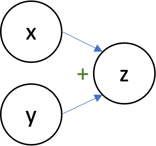
- Each node represents an scalar/vector/tensor/array.
- Edges represent dependencies.
- $y \rightarrow u$ means that $y$ was used to compute $u$
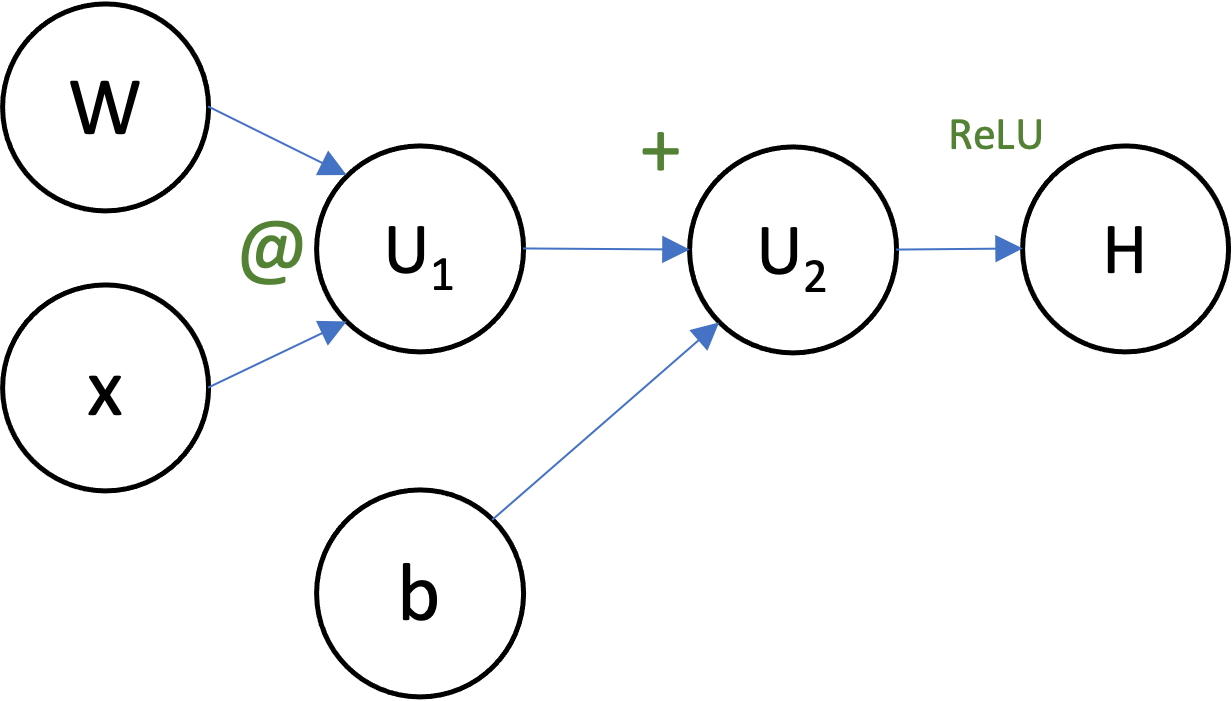
Exercise: Computational Graphs
Can you draw the computational graph for the function
$$H = \max(0, Wx+b)$$for $W \in \mathbb{R}^{c \times d}$, $x \in \mathbb{R}^d$, and $b \in \mathbb{R}^c$?
Backprop in Computational Graphs
To do backprop in a computation represented by a computational graph:
- we first move forward through the graph computing values (in the direction of the arrows),
- then we move backward through the graph accumulating gradients (opposite the direction of the arrows).
Exercise: Backprop
Using your computational graph, suppose that $W = 2$, $x = 3$, and $b = 1$. Write out (in order!) the steps that backprop would to to compute the gradients of $H$ with respect to everything ($W$, $x$, and $b$).
- $U_1 = 2 \cdot 3 = 6$
- $U_2 = U_1 + b = 6 + 1 = 7$
- $H = \operatorname{ReLU}(U_2) = \operatorname{ReLU}(7) = 7$
- $\nabla_H H = \frac{\partial H}{\partial H} = 1$
- $\frac{\partial H}{\partial U_2} = \frac{\partial}{\partial U_2} H(\operatorname{ReLU}(U_2)) = \operatorname{ReLU}'(U_2) \cdot \frac{\partial H}{\partial H} = 1 \cdot 1 = 1$
- $\frac{\partial H}{\partial b} = \frac{\partial}{\partial b} H(U_2(b)) = H'(U_2(b)) \cdot U_2'(b) = \frac{\partial H}{\partial U_2} \cdot \frac{\partial U_2}{\partial b} = 1 \cdot 1 = 1$
- $\frac{\partial H}{\partial U_1} = \frac{\partial H}{\partial U_2} \cdot \frac{\partial U_2}{\partial U_1} = 1 \cdot 1 = 1$
- $\frac{\partial H}{\partial W} = \frac{\partial}{\partial W} H(Wx) = \frac{\partial H}{\partial U_1} \cdot x = 1 \cdot 3 = 3$
- $\frac{\partial H}{\partial x} = \frac{\partial}{\partial x} H(Wx) = \frac{\partial H}{\partial U_1} \cdot W = 1 \cdot 2 = 2$
Exercise 2: Backprop on a non-tree DAG
$$u = x+1 \hspace{2em} y = xu = x(x+1)$$$$x = 17$$Note: $17 \cdot 18 = 306$ (according to ChatGPT)
- $\frac{dy}{dx} \leftarrow 0$
- $u = x + 1 = 17 + 1 = 18$
- $u.\operatorname{grad} \leftarrow 0$
- $y = x u = 17 \cdot 18 = 306$
- $\frac{dy}{dy} \leftarrow 0$
- $\frac{dy}{dy} \leftarrow 1$
- $\frac{dy}{du} \leftarrow \frac{dy}{du} + \frac{dy}{dy} \cdot \frac{d}{du} (xu) = 0 + 1 \cdot x = 17$
- $\frac{dy}{dx} \leftarrow \frac{dy}{dx} + \frac{dy}{dy} \cdot u = 0 + 1 \cdot u = 18$
- $\frac{dy}{dx} \leftarrow \frac{dy}{dx} + \frac{dy}{du} \cdot \frac{d}{dx} (x + 1) = 18 + 17 \cdot 1 = 35$
Advantages/Disadvantages of Backpropagation
Advantages:
- Compute gradients with little (constant-factor) overhead
Disadvantages:
- Memory!
- Need to store a lot of derivatives
- Need to manifest the whole compute graph
- Scheduling questions (how to order)