Recall: "classical" machine learning
- Example-label pairs $(x,y)$
- Example usually contains more information than the label
- e.g. we might process a $1024 \times 1024 \times 3$ image only to produce a single label with $1000$ discrete options
- This is not bad, but it would be nice to have more signal for learning
Modern causal autoregressive learning
- Example is a sequence $(x_1, x_2, \ldots, x_n)$
- Task is to predict $x_k$ given $(x_1, \ldots, x_{k-1})$ for all $k \in \{1,\ldots,n\}$
- For probabilistic sequence modeling with $x_i \in V$ for discrete set $V$ (usually a vocabulary), this results in a density of the form $$\mathbf{P}(x_1, x_2, \ldots, x_n) = \prod_{k = 1}^n p_{w}(x_k \mid x_1, x_2, \ldots, x_{k-1})$$ where $p_w$ denotes the learned model as a function of the weights $w$.
- Minimize the negative-log-likelihood of the data (cross-entropy loss).
- Beneficial consequence: example and "labels" are the same
- they contain the same amount of information
- gives us a lot of "signal" for learning
- e.g. if we process a sequence of length $1024$ then there are $1024$ things we are trying to predict
Drawback of causal autoregressive modeling
- Sampling latency is high due to high memory bandwidth demands (Memory Ops from https://arxiv.org/pdf/2403.14123)
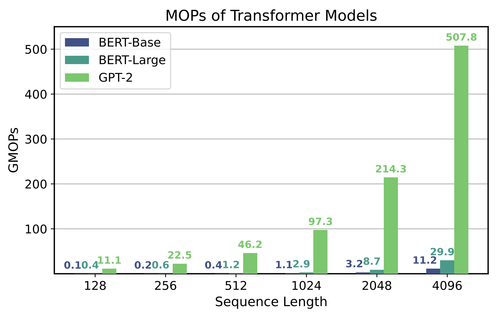
To sample a sequence of length $n$, we need to query the model $n$ times, and each such query requires that we load $w$ $$\text{total mem bw required (not incl. activations)} = n \cdot d_{\text{model}} \cdot (\operatorname{bpw})$$ where $d_{\text{model}}$ is the model size and $\operatorname{bpw}$ is the bytes-per-weight of the (possibly compressed) model.
This becomes intractable if $n$ is very large.
Imagine we tried to do this to predict the pixels in a $1024 \times 1024$ image! Two big problems:
- Attention is quadratic in $n$, and here $n$ would be $1024^2$.
- The memory bandwidth required just to load the weights would be huge: $1024^2 \cdot d_{\text{model}}$.
One Alternative: Diffusion Models
Motivating idea. Instead of modeling our distribution autoregressively, let's do the following
$$\mathbf{P}(x_1, x_2, \ldots, x_n) = \prod_{k = 1}^n p_{w}(x_k).$$Now we can sample all the $x_i$ in parallel, since $x_k$ no longer depends on $x_{<k}$. This means we only need one load of the model weights to do this!
- Memory bandwidth would just be $d_{\text{model}} \cdot (\operatorname{bpw})$
What's the downside of doing this?
Okay, so obviously we can't do that...
What if we did something slightly more clever by augmenting our state space with an extra variable $z_k$ (same shape as $x_k$) which represents some "hint" or "partial" information about what might be at position $k$
$$\mathbf{P}(x_1, x_2, \ldots, x_n) = \sum_{z_1,\ldots,z_n} \prod_{k = 1}^n p_{w}(x_k \mid z_1, \ldots, z_n) \cdot p_{w}(z_k).$$Now the sampling process has two steps:
- Draw $z_1, \ldots, z_n$ in parallel by querying the model
- Draw $w_1, \ldots, w_n$ in parallel conditioned on $(z_1, \ldots, z_n)$
- Memory bandwidth is now $2 \cdot d_{\text{model}} \cdot (\operatorname{bpw})$
We can do this across multiple steps too. Augmenting the space with $z_{k}^{(T)}$ for $k \in \{1,\ldots,n\}$ and $T \in \{1,\ldots,T-1\}$
$$\mathbf{P}(x_1, x_2, \ldots, x_n) = \sum_{z} \prod_{k = 1}^n p_{w,T}(x_k \mid z_1^{(T-1)}, \ldots, z_n^{(T-1)}) \cdot p_{w,T-1}(z_k^{(T-1)} \mid z_1^{(T-2)}, \ldots, z_n^{(T-2)}) \cdots p_{w,2}(z_k^{(2)} \mid z_1^{(1)}, \ldots, z_n^{(1)}) \cdot p_{w,1}(z_k^{(1)}).$$Now the sampling process has $T$ steps:
- Draw $z_1^{(1)}, \ldots, z_n^{(1)}$ in parallel by querying the model
- Draw $z_1^{(2)}, \ldots, z_n^{(2)}$ in parallel by querying the model, conditioned on $(z_1^{(1)}, \ldots, z_n^{(1)})$
- Now we can discard $(z_1^{(1)}, \ldots, z_n^{(1)})$, since we don't need them anymore
- Continue by drawing $z_1^{(3)}, \ldots, z_n^{(3)}$ in parallel by querying the model, conditioned on $(z_1^{(2)}, \ldots, z_n^{(2)})$
- Repeat, eventually producing $z_1^{(T-1)}, \ldots, z_n^{(T-1)}$
- Draw $w_1, \ldots, w_n$ in parallel conditioned on $(z_1^{(T-1)}, \ldots, z_n^{(T-1)})$
- Memory bandwidth is now $T \cdot d_{\text{model}} \cdot (\operatorname{bpw})$
But this is all little awkward. Some questions we'd need to answer:
- Where do we get $z$ from for training? (if we need a value for $z$)
- How to we minimize the loss efficiently? (can't just sum over exponentially many values for $z$ to mimimize the log-likelihood)
The ELBO
Very powerful tool in Bayesian machine learning. Let $X$ and $Z$ be any random variables, and let $p$ be a joint distributions of $X$ and $Z$, and let $q$ be a (possibly different) distribution of $Z$ conditioned on $X$. Then the ELBO ("evidence lower bound") for an example $x$ is defined as
$$\operatorname{ELBO}(x; p, q) = \mathbf{E}_{z \sim q(\cdot \mid x)}\left[ \log \frac{p(x,z)}{q(z|x)} \right].$$It's a standard result that
$$\log p(x) \ge \operatorname{ELBO}(x; p, q).$$Why? Observe that
\begin{align*} \log p(x) &= \log\left( \sum_{z} p(x,z) \right) \\&= \log\left( \sum_{z} q(z|x) \cdot \frac{p(x,z)}{q(z|x)} \right) \\&= \log\left( \mathbf{E}_{z \sim q(\cdot \mid x)}\left[ \frac{p(x,z)}{q(z|x)} \right] \right) \\&\ge \mathbf{E}_{z \sim q(\cdot \mid x)}\left[ \log\left( \frac{p(x,z)}{q(z|x)} \right) \right] \end{align*}where this last step follows from Jensen's inequality. Also, obviously the NELBO ("negative ELBO")
$$-\log p(x) \le -\operatorname{ELBO}(x; p, q) = \operatorname{NELBO}(x; p, q)$$is an upper bound on the loss we'd like to minimize. Main idea: minimize this upper bound!
Training with ELBO Recipe
When we want to minimize the negative log likelihood of some data $X$ but our model gives us a joint distribution of $X$ and $Z$ rather than just a distribution over $X$, we do the following:
- Choose some conditional distribution $q(Z | X)$ — independent of the model weights
- Draw $z$ from that $q$, given $x$
- Let the loss of this example be $\log \frac{p_w(x,z)}{q(z|x)}$
- Backprop and run gradient descent normally
Many problems still!
- We blew up the state by a factor of $T$
- Now the model is trying to predict these random samples $z$ which might not have much information about $x$
- Just kicked the design can down the road: now we still need to pick $q$
We can fix a few of these problems by re-writing the loss
If we let $x$ denote $x_1, \ldots, x_n$ and $z^{(t)}$ denote $z^{(t)}_1, \ldots, z^{(t)}_n$, and we require that $q$ have a Markov-chain structure,
\begin{align*} \operatorname{ELBO}(x) &= \mathbf{E}_{z \sim q(\cdot \mid x)}\left[ \log \frac{p(x,z)}{q(z|x)} \right] \\&= \mathbf{E}_{z \sim q(\cdot \mid x)}\left[ \log\left( \frac{ p_{w,T}(x \mid z^{(T-1)}) \cdot p_{w,T-1}(z^{(T-1)} \mid z^{(T-2)}) \cdots p_{w,2}(z^{(2)} \mid z^{(1)}) \cdot p_{w,1}(z^{(1)}) }{ q(z^{(T-1)} \mid z^{(T-2)}, x) \cdots q(z^{(2)} \mid z^{(1)}, x) \cdot q(z^{(1)} \mid x) }\right) \right] \\&= \mathbf{E}_{z \sim q(\cdot \mid x)}\left[ \log\left( p_{w,T}(x \mid z^{(T-1)}) \right) + \log\left( \frac{ p_{w,T-1}(z^{(T-1)} \mid z^{(T-2)}) }{ q(z^{(T-1)} \mid z^{(T-2)}, x) }\right) + \cdots + \log\left( \frac{ p_{w,1}(z^{(1)}) }{ q(z^{(1)} \mid x) }\right) \right] \\&= \mathbf{E}_{z \sim q(\cdot \mid x)}\left[ \log\left( p_{w,T}(x \mid z^{(T-1)}) \right) \right] + \mathbf{E}_{z \sim q(\cdot \mid x)}\left[ \log\left( \frac{ p_{w,T-1}(z^{(T-1)} \mid z^{(T-2)}) }{ q(z^{(T-1)} \mid z^{(T-2)}, x) }\right) \right] + \cdots + \mathbf{E}_{z \sim q(\cdot \mid x)}\left[ \log\left( \frac{ p_{w,1}(z^{(1)}) }{ q(z^{(1)} \mid x) }\right) \right] \end{align*}Key Trick: Evaluate only one of the terms of this sum, using subsampling (our old trick from the first lecture). A random term of this sum looks like:
$$\mathbf{E}_{z \sim q(\cdot \mid x)}\left[ \log\left( \frac{ p_{w,t}(z^{(t)} \mid z^{(t-1)}) }{ q(z^{(t)} \mid z^{(t-1)}, x) }\right) \right]$$and we can rewrite this as
$$\mathbf{E}_{z_{t-1} \sim q(Z_{t-1} \mid x)}\left[ \sum_{z^{(t)}} q(z^{(t)} \mid z^{(t-1)}, x) \log\left( \frac{ p_{w,t}(z^{(t)} \mid z^{(t-1)}) }{ q(z^{(t)} \mid z^{(t-1)}, x) }\right) \right]$$This gives us a full recipe for a discrete-time, discrete-space diffusion!
Continuous Diffusion
Much real diffusion works in continuous space.
- Make the time coordinate $t$ continuous rather than discrete: making an infinite number of infinitely small changes.
- The "noising" process $q$ is typically Brownian motion, and we think about the whole process as a noising-denoising process where the model $p$ learns to denoise images that had Gaussian noise added to them by $q$
Handling the Quadratic Cost of Attention
We still haven't addressed the fact that attention scales as $\mathcal{O}(n^2)$
Two main ways to solve this:
- More efficient attention layers
- Linear attention
- Sliding window attention
- Structured state-space models
- A combination of recurrent and convolutional neural networks (RNNs and CNNs), which can be efficiently computed as either a recurrence (like an RNN) or a convolution (like a CNN). This means we can efficiently generate one-token-at-at-time for autoregressive modeling (like an RNN) but also process the whole sequence in parallel for efficient training (like a CNN).