So far we've been talking about ways to scale our machine learning pipeline that focus on a single machine. But if we really want to scale up to huge datasets and models, eventually one machine won't be enough. This lecture will cover methods for using multiple machines to do learning.
Distributed computing basics.
Distributed parallel computing involves two or more machines collaborating on a single task by communicating over a network. Unlike parallel programming on a single machine, distributed computing requires explicit (i.e. written in software) communication among the workers.
There are a few basic patterns of communication that are used by distributed programs:
- Push. Machine $A$ sends some data to machine $B$.
- Pull. Machine $B$ requests some data from machine $A$. (This differs from push only in terms of who initiates the communication.)
- Broadcast. Machine $A$ sends some data to many machines $C_1, C_2, \ldots, C_n$.
- Reduce. Compute some reduction (usually a sum) of data on multiple machines $C_1, C_2, \ldots, C_n$ and materialize the result on one machine $B$.
- All-reduce. Compute some reduction (usually a sum) of data on multiple machines $C_1, C_2, \ldots, C_n$ and materialize the result on all those machines $C_1, C_2, \ldots, C_n$.
- Wait. One machine pauses its computation and waits for data to be received from another machine.
Communicating over the network can have high latency, so an important principle of parallel computing is overlapping computation and communication. For the best performance, we want our workers to still be doing useful work while communication is going on (rather than having to stop and wait for the communication to finish).
Running SGD with all-reduce.
All-reduce gives us a simple way of running learning algorithms such as SGD in a distributed fashion. Simply put, the idea is to just parallelize the minibatch. We start with an identical copy of the parameter $w_t$ on each worker. If the SGD update step is $$ w_{t+1} = w_t - \alpha_t \cdot \frac{1}{B} \sum_{b=1}^B \nabla f_{i_{b,t}}(w_t), $$ and there are $M$ worker machines such that $B = M \cdot B'$, then we can re-write this update step as $$ w_{t+1} = w_t - \alpha_t \cdot \frac{1}{M} \sum_{m = 1}^M \frac{1}{B'} \sum_{b=1}^{B'} \nabla f_{i_{m,b,t}}(w_t). $$ Now, we assign the computation of the sum when $m = 1$ to worker $1$, the computation of the sum when $m = 2$ to worker $2$, et cetera. After all the gradients are computed, we can perform the outer sum with an all-reduce operation, after which the full sum $$ \sum_{m = 1}^M \frac{1}{B'} \sum_{b=1}^{B'} \nabla f_{i_{m,b,t}}(w_t) $$ will be present on all the worker machines. From here, each worker can individually compute the new value of $w_{t+1}$ and update its own parameter vector; after this update, the values of the parameters on each worker will be the same. This corresponds to the following algorithm.
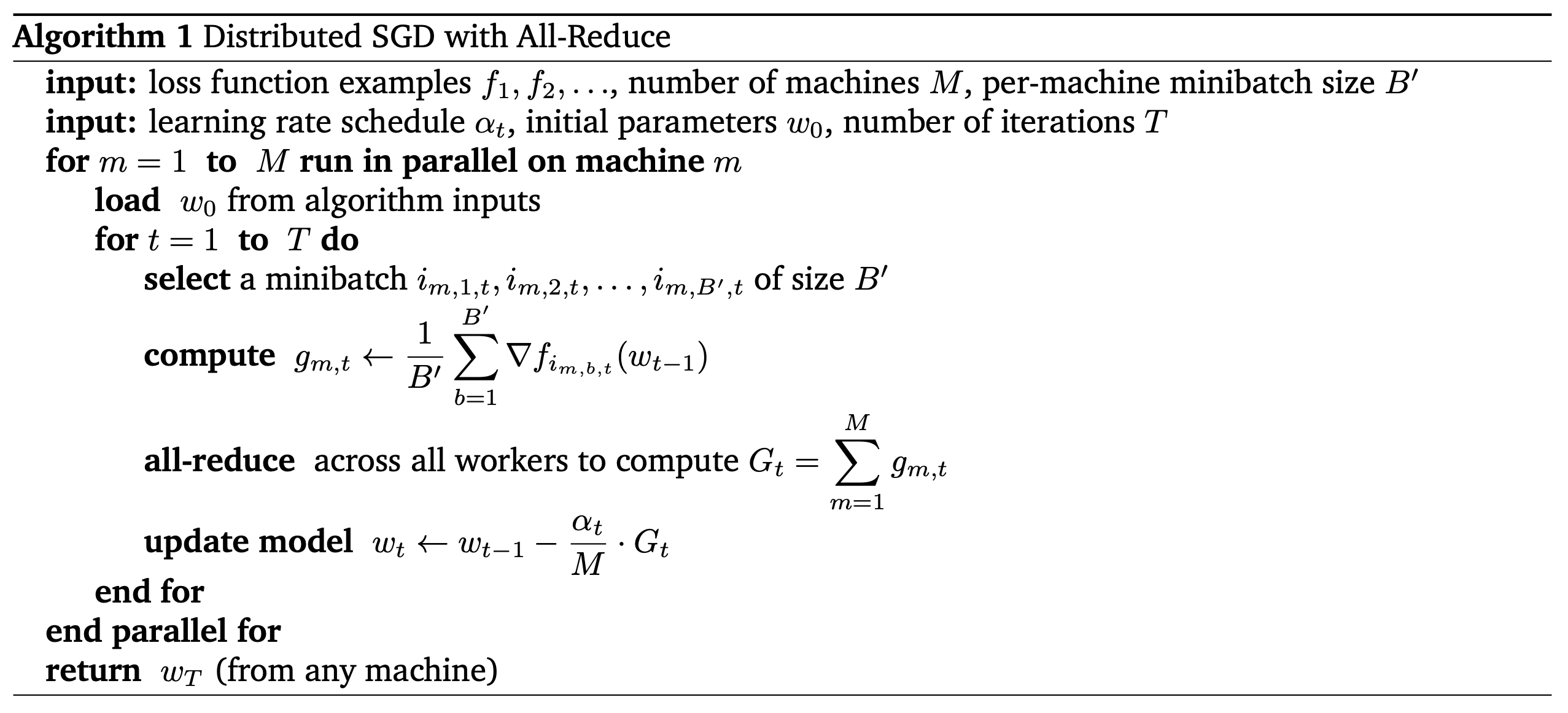
It is straightforward to see how one could use the same all-reduce pattern to run variants of SGD such as Adam and SGD+Momentum.
Benefits of distributed SGD with all-reduce:
- It's easy to reason about, since it's statistically equivalent to minibatch SGD.
- It's easy to implement, since all the worker machines have the same role and it runs on top of standard distributed computing primitives.
Downsides of distributed SGD with all-reduce:
- While the communication for the all-reduce is happening, the workers are (for the most part) idle. We're not overlapping computation and communication.
- The effective minibatch size is growing with the number of machines, and for cases where we \emph{don't} want to run with a large minibatch size for statistical reasons, this can prevent us from scaling to large numbers of machines using this method.
Where do we get the training examples from?
There are two general options for distributed learning:
- Have one or more non-worker servers dedicated to storing the training examples (e.g. a distributed in-memory filesystem), and have the worker machines load training examples from those servers.
- Partition the training examples among the workers themselves and store them locally in memory on the workers.
The parameter server model.
Recall from the early lectures in this course that a lot of our theory talked about the convergence of optimization algorithms. This convergence was measured by some function over the parameters at time $t$ (e.g. the objective function or the norm of its gradient) that is decreasing with $t$, which shows that the algorithm is making progress. For this to even make sense, though, we need to be able to talk about the value of the parameters at time $t$ as the algorithm runs. E.g. in SGD, we had $$ w_{t+1} = w_t - \alpha_t \nabla \tilde \ell_t(w_t) $$ and here $w_t$ is the value of the parameters after $t$ timesteps of the algorithm.
For a program running on a single machine, the meaning of this is usually trivial: the value of the parameters at time $t$ is just the value of some array in the memory hierarchy (backed by DRAM) at that time. But in a distributed setting, there is no shared memory, and communication must be done explicitly. Each machine will usually have one or more copies of the parameters live at any given time, some of which may have been updates less recently than others, especially if we want to do something more complicated than all-reduce. This raises the question: when reasoning about a distributed algorithm, what we should consider to be the value of the parameters a given time?
For SGD with all-reduce, we can answer this question easily, since the value of the parameters is the same on all workers (it's guaranteed to be the same by the all-reduce operation). We just appoint this identical shared value to be the value of the parameters at any given time.
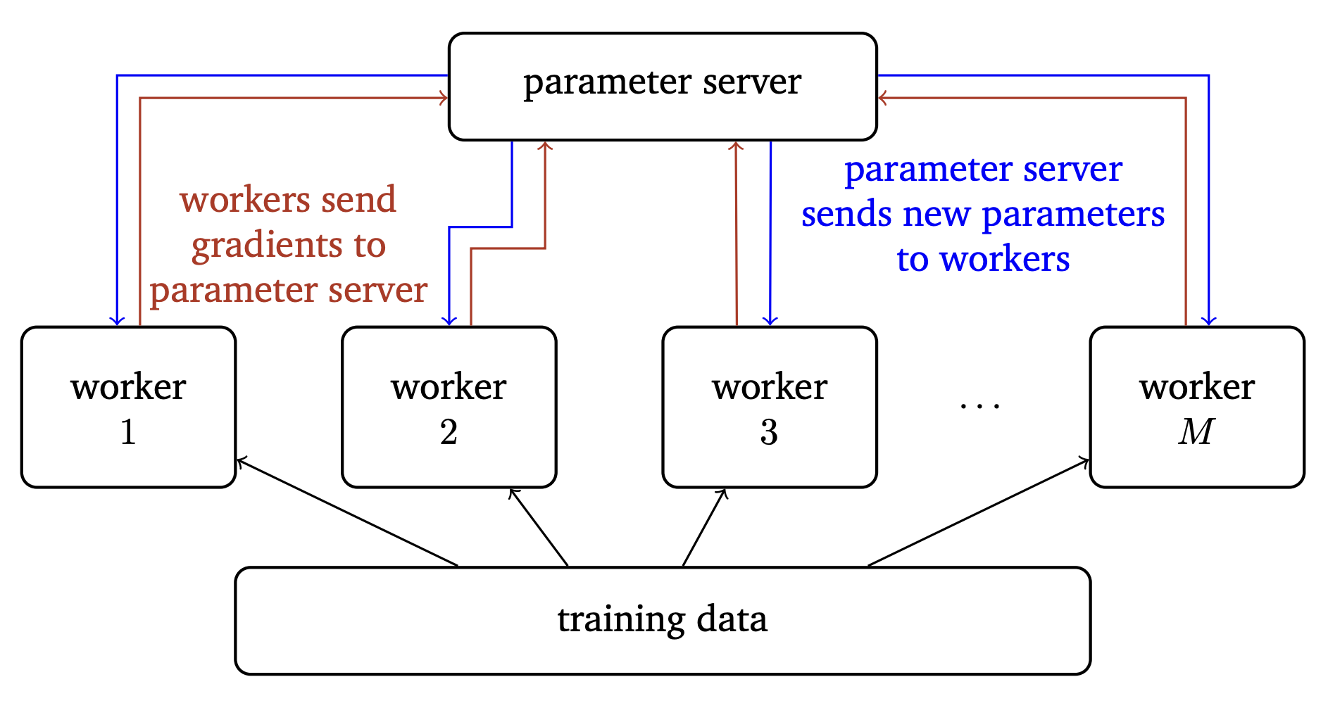
The parameter server model answers this question differently by appointing a single machine, the parameter server, the explicit responsibility of maintaining the current value of the parameters. The most up-to-date gold-standard parameters are the ones stored in memory on the parameter server. The parameter server updates its parameters by using gradients that are computed by the other machines, known as workers, and pushed to the parameter server. Periodically, the parameter server broadcasts its updated parameters to all the other worker machines, so that they can use the updated parameters to compute gradients.
Here is a simple diagram of the parameter server architecture.
Other ways to distribute.
The methods we discussed so far distributed across the minibatch (for all-reduce SGD) and across iterations of SGD (for asynchronous parameter-server SGD). But there are other ways to distribute that are used in practice too.
Distribution for hyperparameter optimization.
- This is something we've already talked about.
- Many commonly used hyperparameter optimization algorithms, such as grid search and random search, are very simple to distribute.
- They can easily be run on a large number of parallel workers to get results faster.
Distribution across the layers of a neural network.
- Main idea: partition the layers of a neural network among different worker machines.
- This makes each worker responsible for a subset of the parameters, and forward and backward signals running through the neural network during backpropagation now also run across the computer network between the different parallel machines.
- This can be particularly useful if the parameters won't fit in memory on a single machine.
- This is very important when we move to specialized machine learning accelerator hardware, where we're running on chips that typically have limited memory and communication bandwidth.
- Common type is \emph{pipeline parallelism} which assigns each layer to one worker machine.
Fully sharded data parallel model.
A hybrid of data-parallel and multi-server parameter server models; works well when memory capacity is limited.
- Shards the model weights across multiple worker machines.
- If there are $m$ workers, then each worker has $1/m$ of the weights of each layer.
- When the cluster goes to compute the forward or backward pass for a layer, it first broadcasts all those weights.
- When gradients are computed, each worker accumulates the part of the gradients corresponding to its shard with a scatter-reduce.