Lecture 13: Scaling Laws

CS4787/5777 --- Principles of Large-Scale Machine Learning Systems

Recall: hyperparameter optimization is expensive!

E.g. https://arxiv.org/pdf/1906.02243

How can we reduce the cost of hyperparameter optimization?

Background: Power Laws

Lots of empirical trends have a power law decay.

$$f(x) = A x^{-\gamma}.$$

import torch
from matplotlib import pyplot
import torchvision

# this is a big dataset tokenized with the llama3 tokenizer
tokens = torch.load('../../../Research/tokenizer/train/0.llama3.pt',weights_only=True)

counts = torch.bincount(tokens)
counts = counts.sort(descending=True).values;

pyplot.plot(counts)
pyplot.ylabel('number of occurrences of token in dataset');
pyplot.xlabel('token rank order');

pyplot.loglog(counts)
pyplot.ylabel('number of occurrences of token in dataset');
pyplot.xlabel('token rank order');

pyplot.loglog(counts, label='empirical frequency')
pyplot.semilogy(2e7 * (1+torch.arange(128000)).float()**(-1.0), label='power law')
pyplot.ylabel('number of occurrences of token in dataset');
pyplot.xlabel('token rank order');
pyplot.legend();

X = train_dataset = torchvision.datasets.MNIST(
                root = './data',
                train = True,
                transform = torchvision.transforms.ToTensor(),
                download = True).data.view(-1,28*28).float()

svdX = torch.linalg.svdvals(X)

X.shape

torch.Size([60000, 784])

pyplot.loglog(svdX, label='empirical')
pyplot.semilogy(5e5 * (1+torch.arange(28*28)).float()**(-0.8), label='power law')
pyplot.ylim((1e2,1e6));
pyplot.title('Singular Values of MNIST Dataset');
pyplot.ylabel('singular value');
pyplot.xlabel('rank order');
pyplot.legend();

n = 1024
Z = torch.randn(n,n)
svdZ = torch.linalg.svdvals(Z)

pyplot.loglog(svdZ)

[<matplotlib.lines.Line2D at 0x14597b6d0>]

pyplot.plot(svdZ)

[<matplotlib.lines.Line2D at 0x154b1fc10>]

Power laws are ubiquitous in machine learning and in science.

Where else have you seen power laws?

"Scaling Laws for Neural Language Models"

Kaplan et. al. 2020

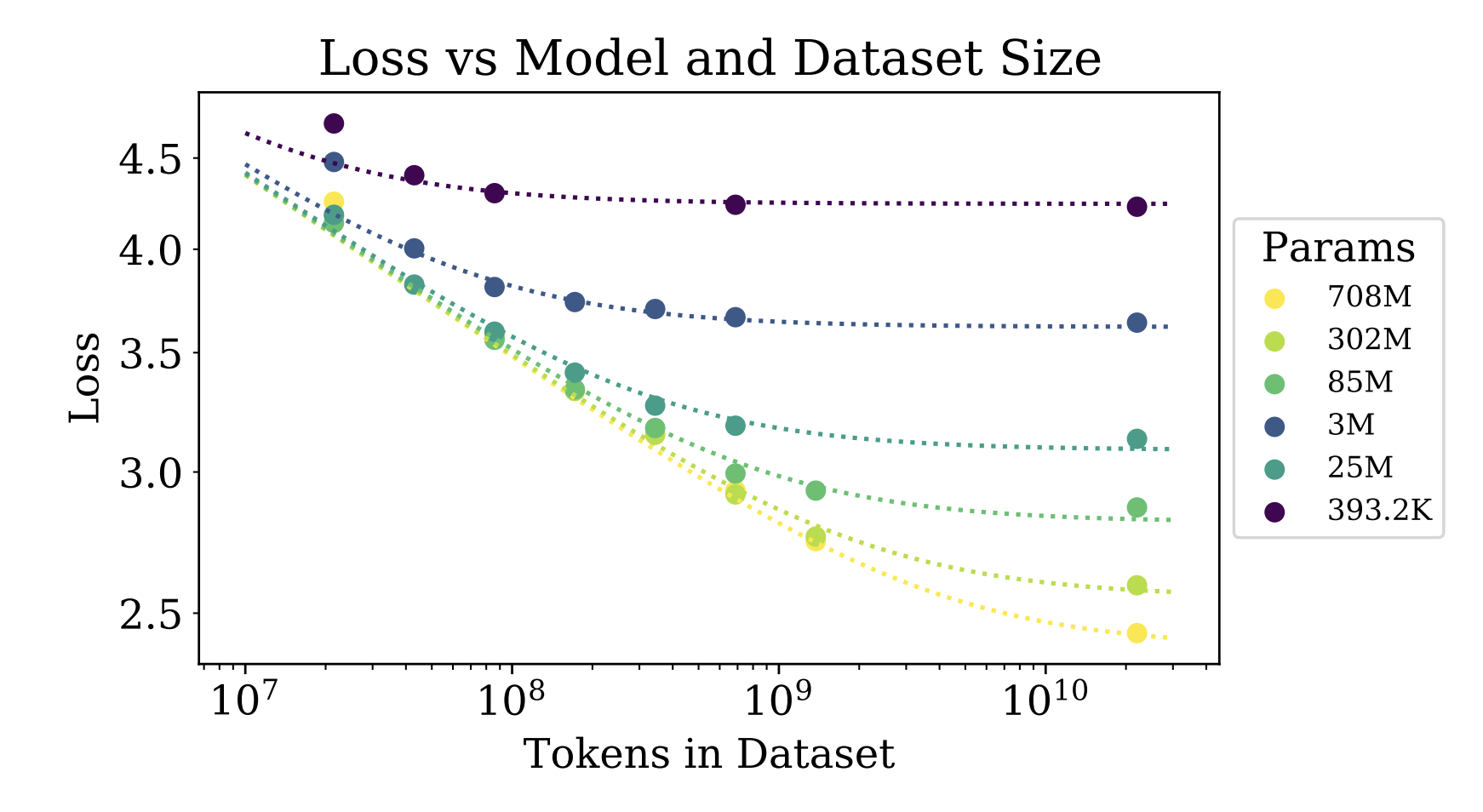
Claim: the Pareto frontier of loss as a function of dataset size, minimizing over model size, scales like a power law.

Abstract is very informative:

We study empirical scaling laws for language model performance on the cross-entropy loss.

The loss scales as a power-law with model size, dataset size, and the amount of compute used for training, with some trends spanning more than seven orders of magnitude. Other architectural details such as network width or depth have minimal effects within a wide range. Simple equations govern the dependence of overfitting on model/dataset size and the dependence of training speed on model size. These relationships allow us to determine the optimal allocation of a fixed compute budget.

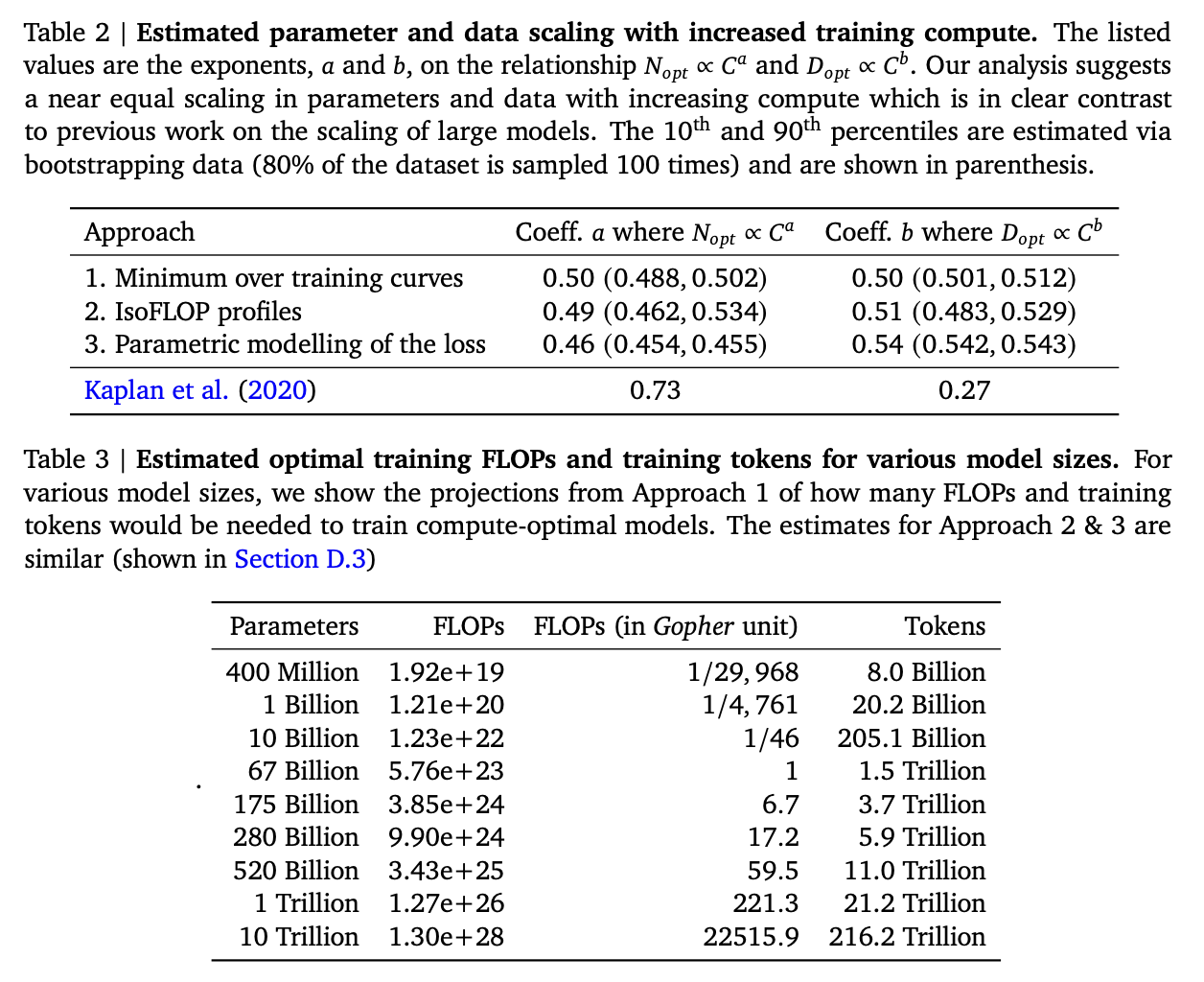
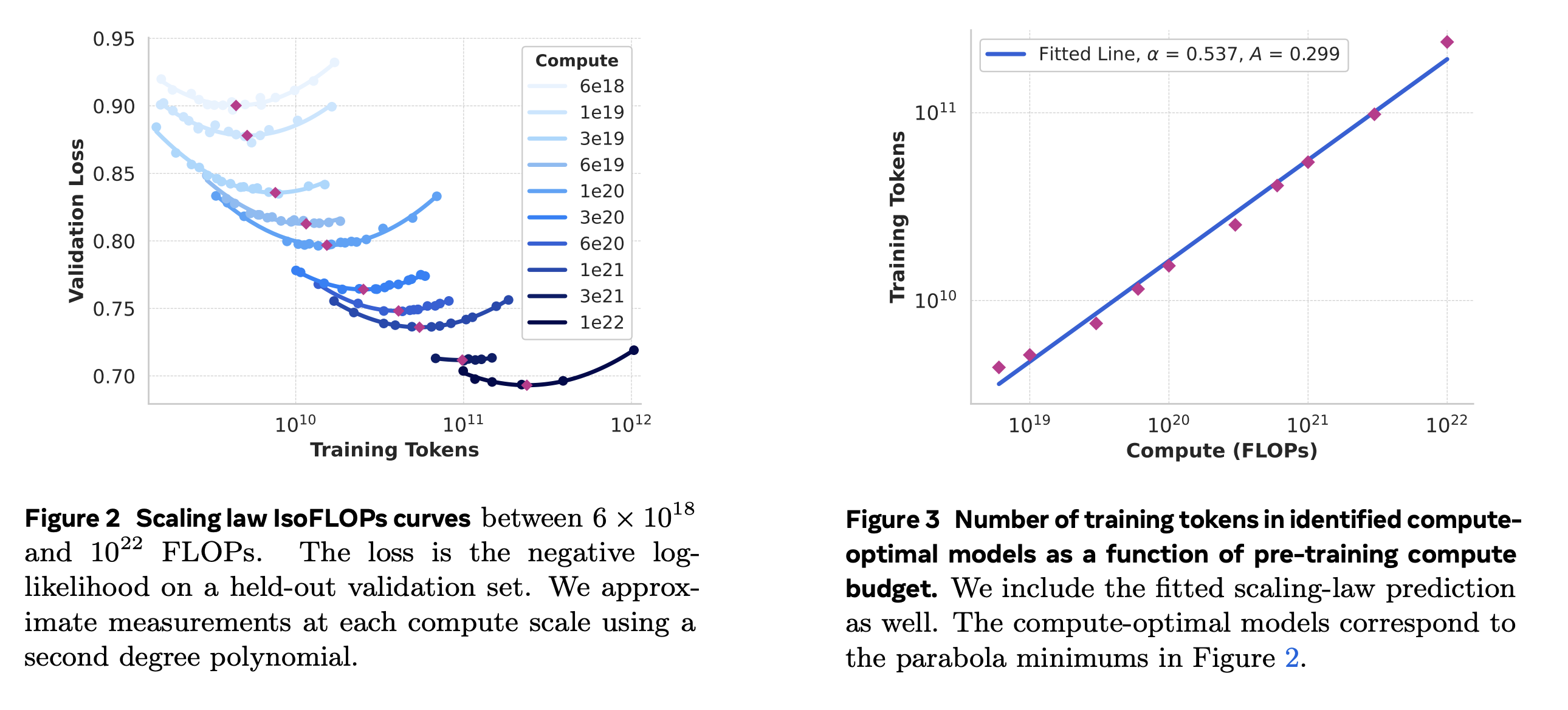
A highly impactful later scaling law: Chinchilla

Suppose we have a transformer model with $N$ parameters, and we train it for one epoch on a dataset with $D$ tokens. Then the loss after training (with "standard" hyperparameters, AdamW, cosine learning rate schedule, etc.) will follow the loss scaling law

$$L(N,D) = \frac{406.4}{N^{0.34}} + \frac{410.7}{D^{0.28}} + 1.69.$$

Data suggests that "results are independent of the dataset as long as one does not train for more than one epoch."

What does this suggest about how we should set these parameters as a function of the number of FLOPs we want to use?

Say that $\operatorname{FLOPs}(N,D) = 6ND = C$. (Why?) What will we get as an optimal assignment?

0.34/(0.34 + 0.28)

0.5483870967741935

0.28/(0.34 + 0.28)

0.45161290322580644

$$N_{\text{opt}} \propto C^{\alpha} \hspace{4em} D_{\text{opt}} \propto C^{\beta}$$

Nowadays, large model pretraining is based on scaling laws

E.g. for Llama3...

Important note: Scaling laws that minimize loss given a training FLOPs budget do not take inference cost into account!

Do we think that increasing focus on inference cost would result in relatively larger $N$? Relatively larger $D$? Neither?