Lecture 4: Backpropagation

CS4787/5777 — Principles of Large-Scale Machine Learning Systems

$\newcommand{\R}{\mathbb{R}}$

Announcements

• Office hour calendar is on the website and on Ed.
• First programming assignment is out.
• First paper reading assignment for CS5777 is out.

Continuing from last time: Forward Mode AD

• Fix one input variable $x$ over $\mathbb{R}$.
• At each step of the computation, as we're computing some value $y$, also compute $\frac{\partial y}{\partial x}$.
• We can do this with a dual numbers approach: each number $y$ is replaced with a pair $(y, \frac{\partial y}{\partial x})$.

Forward Mode AD Takeaways

• Each operation in the original program is replaced with two operations
  • one to compute the value $y$ (same as original)
  • one to compute the derivative $\frac{\partial y}{\partial x}$
• The new operation has an analogous structure to the original one
  • since its the derivative
  • e.g. a matrix multiply would produce a new matrix multiply
• If the original operation had compute cost $C$, the new operation has cost $O(C)$.

Implementing Forward Mode AD

In Python, we can use operator overloading and dynamic typing. Suppose I write a function

def f(x):
    return x*x + 1.0

imagining that we will call it with x being a floating-point number.

• I can still call it with x being a dual number (because Python is not explicitly typed).
• When I do this, the operators * and + desugar to calls to my __mul__ and __add__ methods.
• I can do the differentiation in these methods.
• I can do this across the whole program to differentiate compositions of functions!

Benefits of Forward Mode AD

• Simple in-place operations
• Easy to extend to compute higher-order derivatives
• Only constant factor increase in memory use, since each $\frac{\partial y}{\partial x}$ object is the same size as $y$ and is only live when $y$ is

Problems with Forward Mode AD

• Differentiate with respect to one input
  • problematic for ML, where we usually want to compute gradients
  • If we are computing a gradient of $f: \mathbb{R}^d \rightarrow \mathbb{R}$, blow-up proportional to the dimension $d$

Reverse-Mode AD

• Fix one output $\ell$ over $\mathbb{R}$
• Compute partial derivatives $\frac{\partial \ell}{\partial y}$ for each value $y$
• Need to do this by going backward through the computation

Problem: can't just compute derivatives as-we-go like with forward mode AD.

Backpropagation: The usual type of Reverse-AD we use

Same as before: we replace each number/array $y$ with a pair, except this time the pair is not $(y, \frac{\partial y}{\partial x})$ but instead $(y, \nabla_y \ell)$ where $\ell$ is one fixed output.

• I use $\ell$ here because usually in ML the output is a loss.
• Observe that $\nabla_y \ell$ always has the same shape as $y$.

Deriving Backprop from the Chain Rule

Suppose that the output $\ell$ can be written as $$\ell = f(u), \; u = g(y).$$ Here, $g$ represents the immediate next operation that consumes the intermediate value $y$ (producing a new intermediate $u$), and $f$ represents all the rest of the computation. Suppose all these expressions are scalars. By the chain rule, $$\frac{\partial \ell}{\partial y} = g'(y) \cdot \frac{\partial \ell}{\partial u}.$$ That is, we can compute $\frac{\partial \ell}{\partial y}$ using only "local" information (information that's available in the program around where $y$ is computed and used) and $\frac{\partial \ell}{\partial u}$.

Deriving Backprop from the Chain Rule

More generally, suppose that the output $\ell$ can be written as $$\ell = F(u_1, u_2, \ldots, u_k), \; u_i = g_i(y).$$ Here, the $g_1, g_2, \ldots, g_k$ represent the immediate next operations that consume the intermediate value $y$ (note that there may be many such $g$), the $u_i$ are the arrays output by those operations, and $F$ represents all the rest of the computation. By the multivariate chain rule, $$\nabla_y \ell = \sum_{i=1}^k D g_i(y)^T \nabla_{u_i} \ell.$$ Again, we see that we can compute $\frac{\partial \ell}{\partial y}$ using only "local" information and the gradients of the loss with respect to each array that immediately depends on $y$, i.e. $\nabla_{u_i} \ell$.

When can we compute the gradient with respect to $y$?

• Not immediately when we compute $y$.
• Not until after we've computed the gradient with respect to every other array/tensor that $y$ was used to compute.

Idea: remember the order in which we computed all the intermediate arrays/tensors, and then compute their gradients in the reverse order.

When can we start computing the gradient with respect to $y$?

$$\nabla_y \ell = \sum_{i=1}^k D g_i(y)^T \nabla_{u_i} \ell.$$

• The gradient with respect to $y$ is a sum of a bunch of components, one for each array/tensor that immediately depends on $y$.
• We can compute each element of that sum as soon as we know the gradient with respect to the corresponding tensor.

High-level BP algorithm:

• For each array/tensor, initialize a gradient "accumulator" to 0. Set the gradient of $\ell$ with respect to itself to $1$.
• For each array/tensor $u$ in reverse order of computation, for each array/tensor $y$ on which $u$ depends, compute $D_y u^T \nabla_{u} \ell$ and add it to $y$'s gradent accumulator.
  • Once this step is called for $y$, its gradient will be fully manifested in its gradient accumulator.

Suppose $u \in \mathbb{R}^n$ and $y \in \mathbb{R}^m$. Then $D_y u \in \mathbb{R}^{n \times m}$ and $(D_y u)^T \in \mathbb{R}^{m \times n}$. And note that $\nabla_{u} \ell \in \mathbb{R}^n$

When can we start computing the gradient with respect to $y$?

$$\underbrace{\nabla_y \ell}_{\text{this is used when we process y}} = \sum_{i=1}^k \underbrace{D g_i(y)^T \nabla_{u_i} \ell}_{\text{this is computed when we process $u_i$}}.$$

• Since all the $u_i$ were computed after $y$...
• ...because the $u_i$ depend on $y$...
• ...if we process the gradients in the reverse order, this will work!

But how can we do this?

• Ordinary numbers in a program don't keep track of what they were computed "from"
• Ordinary numbers in a program don't keep track of the order in which they were computed

Computational Graphs

$$z = x + y$$

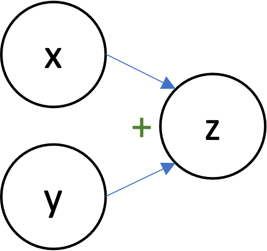
• Each node represents an scalar/vector/tensor/array.
• Edges represent dependencies.
  • $y \rightarrow u$ means that $y$ was used to compute $u$

Exercise: Computational Graphs

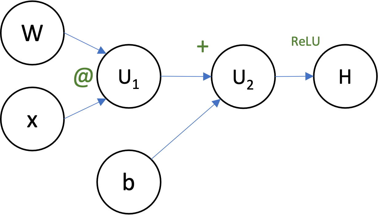
Can you draw the computational graph for the function

$$H = \max(0, Wx+b)$$

for $W \in \mathbb{R}^{c \times d}$, $x \in \mathbb{R}^d$, and $b \in \mathbb{R}^c$?

Backprop in Computational Graphs

To do backprop in a computation represented by a computational graph:

• we first move forward through the graph computing values (in the direction of the arrows),
• then we move backward through the graph accumulating gradients (opposite the direction of the arrows).

Exercise: Backprop

Using your computational graph, suppose that $W = 2$, $x = 3$, and $b = 1$. Write out (in order!) the steps that backprop would to to compute the gradients of $H$ with respect to everything ($W$, $x$, and $b$).

• $U_1= W * x = 2 * 3 = 6$
• $U_2 = U_1 + b = 6 + 1 = 7$
• $H = \operatorname{ReLU}(U_2) = \operatorname{ReLU}(7) = 7$
• $\nabla_H H = 1$
• initialize \nabla_{U_2} H = \nabla_{U_1} H = \nabla_W H = \nabla_x H = \nabla_b H = 0
• $\nabla_{U_2} H += \operatorname{ReLU}'(U_2) \nabla_H H = 1 * 1 = 1$
• $\nabla_{U_1} H += \nabla_{U_2} H = 1$
• $\nabla_{b} H += \nabla_{U_2} H = 1$
• $\nabla_{W} H += x \nabla_{U_1} H = 3 * 1 = 3$
• $\nabla_{x} H += W \nabla_{U_1} H = 2 * 1 = 2$

Advantages/Disadvantages of Backpropagation

$$F(u,v) = uv$$$$\ell = F(x,x)$$$$\frac{d \ell}{d x} = \frac{dF}{du} \cdot \frac{du}{dx} + \frac{dF}{dv} \cdot \frac{dv}{dx}$$$$\frac{d \ell}{d x} = v \cdot 1 + u \cdot 1$$$$\frac{d \ell}{d x} = v + u = x + x = 2x$$

Advantages:

• Compute gradients with little (constant-factor) overhead

Disadvantages:

• Memory!
  • Need to store a lot of derivatives
  • Need to manifest the whole compute graph
• Scheduling questions (how to order)