The Course So Far
So far, we've looked at how to train models efficiently at scale, how to use capabilities of the hardware such as parallelism to speed up training, and even how to run inference efficiently.
However, all of this has been in the context of so-called "batch learning" (also known as the traditional machine learning setup).
In ML theory, this corresponds to the setting of PAC learning (probably approximately correct learning).
PAC Learning (Roughly)
This is the classic ML pipeline setup.
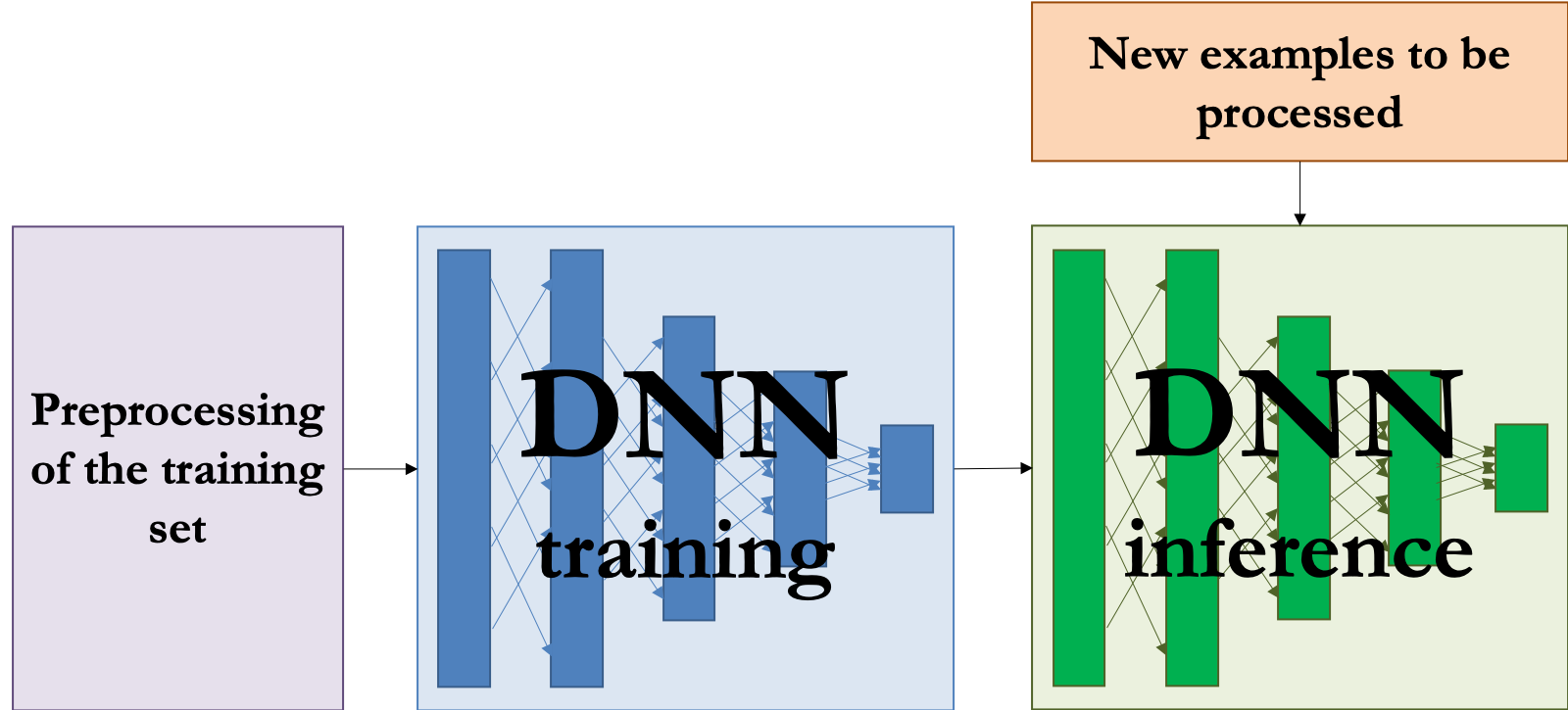
There is typically some fixed dataset $\mathcal{D}$ of labeled training examples $(x,y)$, and we assume it is drawn from the same population that we will be using the model to make predictions on
This dataset is cleaned and preprocessed, then split into a training set, a validation set, and a test set.
An ML model is trained on the training set using some large-scale optimization method (or other method), using the validation set to evaluate and set hyperparameters.
The trained model is then evaluated once on the test set to see if it performs well.
- The system is evaluated only after all learning is completed.
The trained model is possibly compressed for efficient deployment and inference.
Finally, the trained model is deployed and used for whatever task it is intended. Importantly, once deployed, the model does not change!
- Only after learning is completed is the trained model used for inference.
PAC Learning More Formally
Formally, in ML theory, PAC learning is defined in terms of whether a problem class/hypothesis class is PAC learnable i.e. whether it can be learned by a learning algorithm under the PAC learning setup. For classification, this boils down to the claim that:
- there is some algorithm $\mathcal{A}$
- such that for any $\epsilon, \delta > 0$,
- there exists some training set size $n$
- such that if we run $\mathcal{A}$ on a random training set of size at least $n$ (drawn independently from the population associated with the problem), then
- with probability at least $1 - \delta$, the expected error on new examples drawn from the same population will be at most $\epsilon$.
That is, by increasing the size of the training set, we can achieve arbitrarily low error with arbitrarily high probability.
- This is why it is called "Probabilistically Approximately-Correct" Learning.
This batch learning setting is not the only setting in which we can learn, and not the only setting in which we can apply our principles!
Do we really need to separate learning and inference like we do in the batch learning/PAC learning setting?

Online learning
Online learning is a different setting, where learning and inference are interleaved rather than happening in two separate phases.
Online learning on a population with distribution $\mathcal{D}$ works by looping the following steps:
- A new labeled example $(x_t,y_t)$ is sampled from $\mathcal{D}$.
- The learner is given the example $x_t$ and must make a prediction $\hat y_t = h_{w_t}(x_t)$.
- The learner is penalized by some loss function $\ell(\hat y_t, y_t)$.
The learner is given the label $y$ and can now update its model parameters $w_t$ using $(x,y)$ to produce a new vector of parameters $w_{t+1}$ to be used at the next timestep.
- Sometimes in practice, the learner does not get the label $y$ immediately but rather a short time later.
Online learning metrics
With the batch learning setup, we often train by minimizing the training loss and evaluate by looking at the validation error/loss and test error/loss. All these metrics are inherently a function of batches i.e. bulk datasets...How does this translate to the online learning setting where we do not have batches?
One way to state the goal of online learning is to minimize the regret.
For any fixed parameter vector $w$ and number of examples $T$, the regret relative to $h_w$ is defined to be the worst-case extra loss incurred by not consistently predicting using the parameters $w$, that is
$$R(w, T) = \sup_{(x_1,y_1), \cdots, (x_T, y_T)} \; \left( \sum_{t=1}^T \ell(\hat y_t, y_t) - \sum_{t=1}^T \ell(h_w(x_t), y_t) \right),$$where $\hat y_t$ is the prediction actually made by the learning algorithm on this dataset at iteration $t$. The regret relative to the entire hypothesis class is the worst-case regret relative to any assignment of the parameters, $$R(T) = \sup_w R(w, T) = \sup_{(x_1,y_1), \cdots, (x_T, y_T)} \; \left( \sum_{t=1}^T \ell(\hat y_t, y_t) - \inf_w \sum_{t=1}^T \ell(h_w(x_t), y_t) \right).$$ You may recognize this last infimum as looking a lot like empirical risk minimization! We can think about the regret as being the amount of extra loss we incur by virtue of learning in an online setting, compared to the training loss we would have incurred from solving the ERM problem exactly in the batch setting.
What are some applications where we might want to use an online learning setup rather than a traditional batch learning approach?
Algorithms for Online Learning
One popular algorithm for online learning that is very similar to what we've discussed so far is online gradient descent.
It's exactly what it sounds like.
At each step of the online learning loop, it runs $$w_{t+1} = w_t - \alpha \nabla_{w_t} \ell(h_{w_t}(x_t), y_t).$$
This should be very recognizable as the same type of update loop as we used in SGD!
- And we should be able to use most of the techniques we discussed in this course to make it scalable.
In fact, we can use pretty much the same analysis that we used for SGD to bound the regret.
Online Gradient Descent Convergence
Assume that each of the functions $f_t(w) = \ell(h_w(x_t), y_t)$ is convex, no matter what example $(x_t, y_t)$ is chosen. We can equivalently write this as $$f_t(w) - f_t(v) \le \nabla f_t(w)^T (w - v).$$ (This is just the first-order definition of a convex function, and says that the function lies above the tangent line to the function at any point. It is equivalent to...) $$f_t(v) \ge f_t(w) + \nabla f_t(w)^T (v - w).$$
Suppose that we are at the $t$th iteration and the current parameter value is $w_t$. Then for any possible parameter value $\hat w$, the squared-distance to $\hat w$ at the next timestep will be \begin{align*} \norm{ w_{t+1} - \hat w }^2 &= \norm{ w_t - \alpha \nabla f_t(w_t) - \hat w }^2 \ &=
\norm{ w_t - \hat w }^2
-
2 \alpha (w_t - \hat w)^T \nabla f_t(w_t)
+
\alpha^2 \norm{ \nabla f_t(w_t) }^2 \\
&\le
\norm{ w_t - \hat w }^2
-
2 \alpha \left( f_t(w_t) - f_t(\hat w) \right)
+
\alpha^2 \norm{ \nabla f_t(w_t) }^2.
\end{align*} Here, in the last line we applied our inequality from the fact that $f_t$ is convex.
Next, if we sum this up across $T$ total steps, we get \begin{align*} \sum{t=1}^T \norm{ w{t+1} - \hat w }^2 &\le
\sum_{t=1}^T \norm{ w_t - \hat w }^2
-
2 \alpha \sum_{t=1}^T \left( f_t(w_t) - f_t(\hat w) \right)
+
\alpha^2 \sum_{t=1}^T \norm{ \nabla f_t(w_t) }^2.
\end{align*}
This is equivalent to \begin{align*} \norm{ w{t+1} - \hat w }^2 + \sum{t=2}^{T} \norm{ w_t - \hat w }^2 &\le \norm{ w_1 - \hat w }^2 +
\sum_{t=2}^T \norm{ w_t - \hat w }^2
-
2 \alpha \sum_{t=1}^T \left( f_t(w_t) - f_t(\hat w) \right)
+
\alpha^2 \sum_{t=1}^T \norm{ \nabla f_t(w_t) }^2.
\end{align*}
Canceling out all by the non-overlapping terms from the first two sums, and moving the terms about, gives us \begin{align*} 2 \alpha \sum_{t=1}^T \left( f_t(w_t) - f_t(\hat w) \right) &\le
\norm{ w_1 - \hat w }^2
-
\norm{ w_{T+1} - \hat w }^2
+
\alpha^2 \sum_{t=1}^T \norm{ \nabla f_t(w_t) }^2 \\
&\le
\norm{ w_1 - \hat w }^2
+
\alpha^2 \sum_{t=1}^T \norm{ \nabla f_t(w_t) }^2.
\end{align*} And dividing by $2 \alpha$, $$\sum_{t=1}^T \left( f_t(w_t) - f_t(\hat w) \right) \le \frac{1}{2 \alpha} \norm{ w_1 - \hat w }^2 + \frac{\alpha}{2} \sum_{t=1}^T \norm{ \nabla f_t(w_t) }^2.$$
The first expression on the left can be seen to be close to $\alpha$ times the regret, since \begin{align*} R(\hat w, T) &= \sup_{(x_1,y_1), \cdots, (x_T, y_T)} \; \left( \sum_{t=1}^T \ell(\hat y_t, y_t) - \sum_{t=1}^T \ell(h_{\hat w}(x_t), y_t) \right) \\&= \sup_{(x_1,y_1), \cdots, (x_T, y_T)} \; \left( \sum_{t=1}^T \ell(h_{w_t}(x_t), y_t) - \sum_{t=1}^T \ell(h_{\hat w}(x_t), y_t) \right) \\&= \sup_{(x_1,y_1), \cdots, (x_T, y_T)} \; \left( \sum_{t=1}^T f_t(w_t) - f_t(\hat w) \right). \end{align*} And since the above analysis was done for any samples $(x_t,y_t)$, it follows that $$ R(\hat w, T) \le \frac{\norm{ w_1 - \hat w }^2}{2 \alpha} + \frac{\alpha}{2} \sum_{t=1}^T \norm{ \nabla f_t(w_t) }^2.$$
If we add the additional assumptions that
(1) we are limiting the range of parameter vectors we are learning over to a region of diameter at most $D$
- this requires a little bit of tinkering in practice to project back onto that region if we ever go outside it, but here for simplicity we'll ignore that
(2) the magnitude of the gradients is always at most $G$, i.e. $\norm{\nabla f_t(w)} \le G$,
then we can say something about the regret relative to the entire hypothesis class:
$$R(T) \le \sup_{\hat w} \; R(\hat w, T) \le \frac{D^2}{2 \alpha} + \frac{\alpha}{2} \cdot T \cdot G^2.$$And now if we pick step size to minimize this of
$$\alpha = \frac{D}{G \cdot \sqrt{T}} = \mathcal{O}\left(\frac{1}{\sqrt{T}}\right),$$then
$$R(T) \le D G \sqrt{T} = \mathcal{O}\left( \sqrt{T} \right).$$Interpreting this result.
In the online setting, regret grows naturally with time in a way that is very different from loss in the batch setting. If we look at the definition of regret, at each timestep it's adding a new component $$ \ell(\hat y_t, y_t) - \ell(h_w(x_t), y_t) $$ which tends to be positive for an optimally-chosen $w$.
For this reason, we can't expect the regret to go to zero as time increases: the regret will be increasing with time, not decreasing.
Instead, for online learning we generally want to get what's called sublinear regret: a regret that grows sublinearly with time.
Equivalently, we can think about situations in which the average regret $$ \frac{R(T)}{T} = \frac{1}{T} \sum_{t=1}^T \ell(\hat y_t, y_t) - \inf_w \frac{1}{T} \sum_{t=1}^T \ell(h_w(x_t), y_t) $$ goes to zero. We can see that this happens in the case of online gradient descent, where $$ R(T) = O(\sqrt{T}) = o(T). $$
Making online learning scalable.
Most of the techniques we've discussed in class are readily applicable to the online learning setting.
- For example, we can easily define minibatch versions of online gradient descent,
- use adaptive learning rate schemes,
- and even use hardware techniques like parallelism and low precision.
If you're interested in more details about how to do this, there are a lot of papers in the literature.
Many online-setting variants of SGD are subject to ongoing active research, particularly the question of how we should build end-to-end systems and frameworks to support online learning.
Applications of online learning: learning in real time.
A major application of online learning is to deal with real-time streams of data where we want to simultaneously
- Learn from the data as we observe it, and
- Make predictions to drive some real-time decisions.
Online learning algorithms let us naturally update our models to "follow" small changes in the data distribution over time.
- This is great for applications where new classes of examples may arise over small time intervals.
- Also very good for robots adapting to new environments.
- Particularly exciting because it seems to match how humans learn!

A classic example of this is spam detection.
Of course, for a spam detection system to be useful for spam filtering, it needs to make predictions about what emails are spam, and it needs to make those predictions in real time.
But it also needs to learn from new spam emails, so that it can quickly adapt to new patterns in spam.
- Spam email patterns change continuously over time, and we don't want to have to have a human in the loop to retrain a model in response to changes in spam patterns.
What problems might we encounter when trying to do spam detection in an online learning setting?