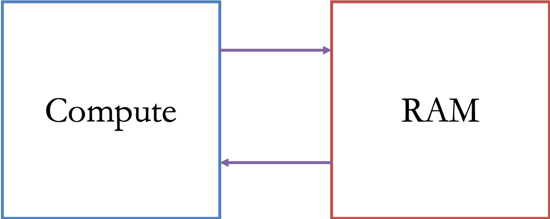
Last time we talked about parallel computing in machine learning, which allows us to take advantage of the parallel capabilities of our hardware to substantially speed up training and inference.
This is an instance of the general principle: Use algorithms that fit your hardware, and use hardware that fits your algorithms.
But compute is only half the story of making algorithms that fit the hardware.
How data is stored and accessed can be just as important as how it is processed.
This is especially the case for machine learning tasks, which often run on very large datasets that can push the limits of the memory subsystem of the hardware.
Today, we'll be talking about how memory affects the performance of the machine learning pipeline.
How do modern CPUs handle memory?
CPUs have a deep cache hierarchy. In fact, many CPUs are mostly cache by area.
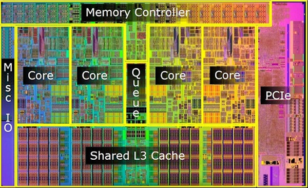
The motivation for this was the ever-increasing gap between the speed at which the arithmetic units on the CPU could execute instructions and the time it took to read/write data to system memory.
Without some faster cache to temporarily store data, the performance of the CPU would be bottlenecked by the cost of reading and/or writing to RAM after every instruction.
But CPUs also have caches
Caches are small and fast memories that are located physically on the CPU chip, and which mirror data stored in RAM so that it can be accessed more quickly by the CPU.
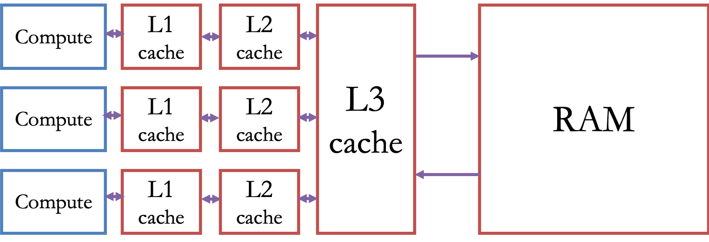
The usual setup of memory on a CPU
a fast L1 cache (typically about 32KB) on each core
a somewhat slower, but larger L2 cache (e.g. 256 KB) on each core
an even slower and even larger L3 cache (e.g. 2 MB/core) shared among cores
DRAM — off-chip memory
Persistent storage — a hard disk or flash drive
A model of a multi-socket computer
Multiple CPU chips on the same motherboard communicate with each other through physical connections on the motherboard.
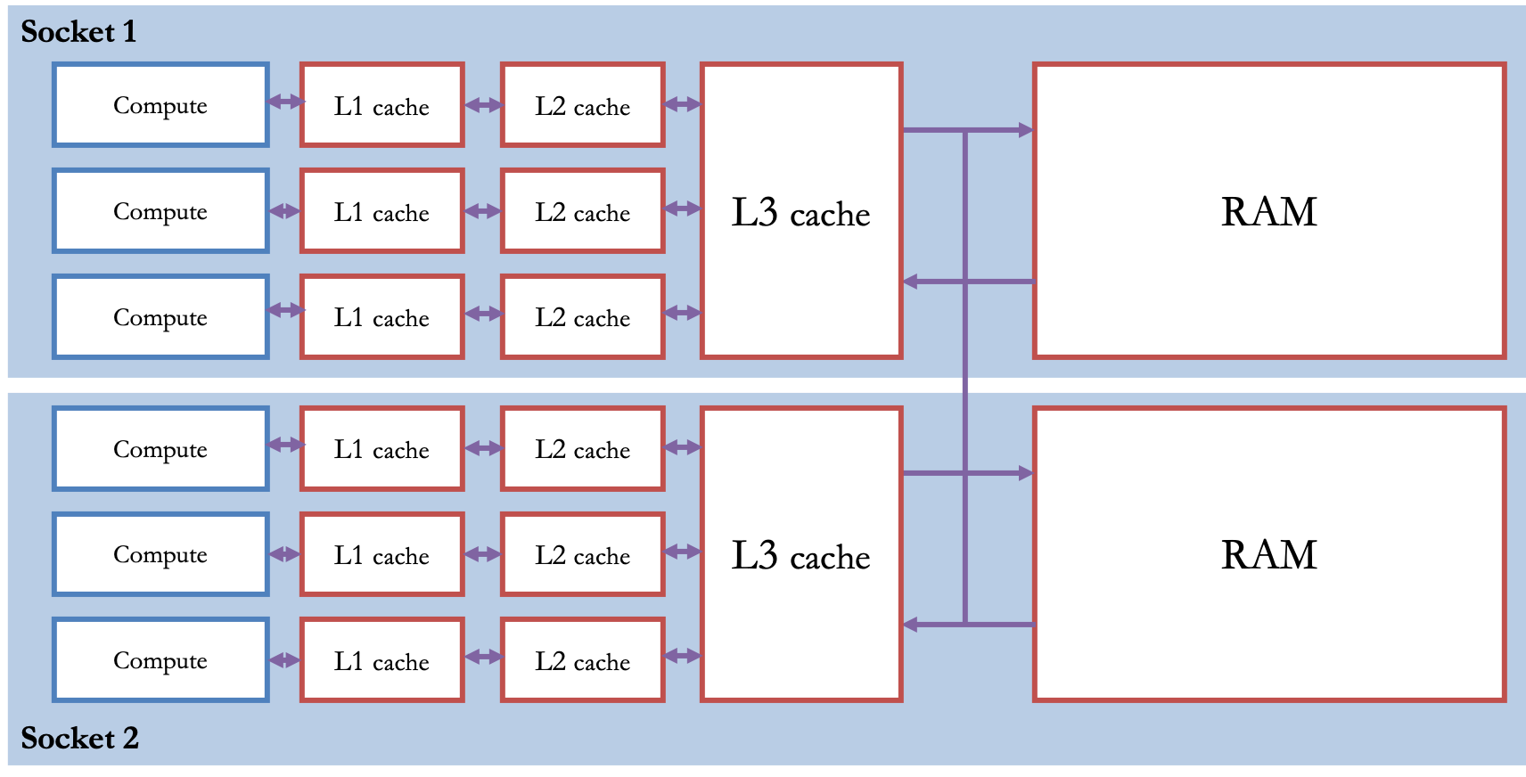
The full view across multiple machines
Multiple CPU chips on the same motherboard communicate with each other through physical connections on the motherboard.
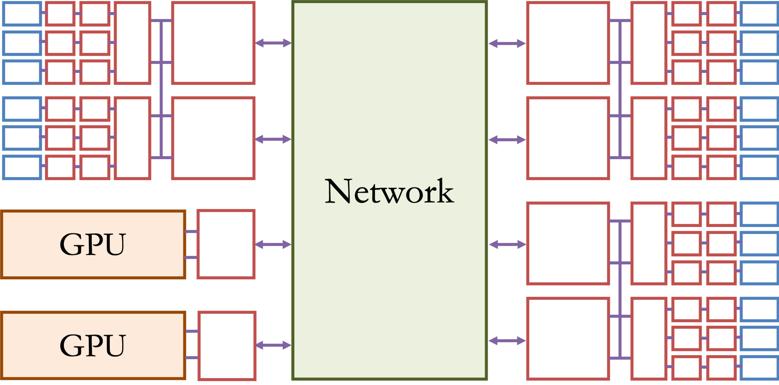
One important thing to notice here:
As we zoom out, much more of this diagram is "memory" boxes than compute boxes.
Hand-wavy consequence: as we scale up, the effect of memory becomes more and more important.
Another important take-away:
Memory has a hierarchical structure
Memories lower in the hierarchy are faster, but smaller
Memories higher in the hierarchy are larger, but slower, and are often shared among many compute units
Two ways to measure performance of a part of the memory hierarchy.
Latency: how much time does it take to access data at a new address in memory?
Throughput (a.k.a. bandwidth): how much data total can we access in a given length of time?
We saw these metrics earlier when evaluating the effect of parallelism.
Ideally, we'd like all of our memory accesses to go to the fast L1 cache, since it has high throughput and low latency.
What prevents this from happening in a practical program?
Result: the hardware needs to decide what is stored in the cache at any given time.
It wants to avoid, as much as possible, a situation in which the processor needs to access data that's not stored in the cache—this is called a cache miss.
Hardware uses two heuristics:
The principle of temporal locality: if a location in memory is accessed, it is likely that that location will be accessed again in the near future.
The principle of spatial locality: if a location in memory is accessed, it is likely that other nearby locations will be accessed in the near future.
Memory Locality
Temporal locality and spatial locality are both types of memory locality.
We say that a program has good spatial locality and/or temporal locality and/or memory locality when it conforms to these heuristics.
When a program has good memory locality, it makes good use of the caches available on the hardware.
In practice, the throughput of a program is often substantially affected by the cache, and can be improved by increasing locality.
Prefetching
A third important heuristic used by both the hardware and the compiler to improve cache performance is prefetching.
Prefetching loads data into the cache before it is ever accessed, and is particularly useful when the program or the hardware can predict what memory will be used ahead of time.
Question: What can we do in the ML pipeline to increase locality and/or enable prefetching?
Access training exmaples in the order they appear in memory
- Prefetch the training examples (prefetch the ones we're going to be using next)
Efficient matrix multiplications
DEMO
A matrix multiply of $A \in \mathbb{R}^{m \times n}$ and $B \in \mathbb{R}^{n \times p}$, producing output $C \in \mathbb{R}^{m \times p}$, can be written by running
$$ C_{i,k} \mathrel{+}= A_{i,j} \cdot B_{j,k} $$for each value of $i \in \{1, \ldots, m\}$, $j \in \{1, \ldots, n\}$, and $k \in \{1, \ldots, p\}$. The natural way to do this is with three for loops. But what order should we run these loops? And how does the way we store $A$, $B$, and $C$ affect performance?
using Libdl # open a dynamic library that links to the C code
tm_lib = Libdl.dlopen("demo/test_memory.lib");
function test_mmpy(loop_order::String, Amaj::String, Bmaj::String, Cmaj::String, m, n, p, num_runs)
    @assert(loop_order in ["ijk","ikj","jki","jik","kij","kji"])
    @assert(Amaj in ["r","c"])
    @assert(Bmaj in ["r","c"])
    @assert(Cmaj in ["r","c"])
    f = Libdl.dlsym(tm_lib, "test_$(loop_order)_A$(Amaj)B$(Bmaj)C$(Cmaj)")
    ccall(f, Float64, (Int32, Int32, Int32, Int32), m, n, p, num_runs)
end
d = 512;
num_runs = 10;
measurements = []
for loop_order in ["ijk","ikj","jki","jik","kij","kji"]
    for Am in ["r","c"]
        for Bm in ["r","c"]
            for Cm in ["r","c"]
                push!(measurements, (loop_order * "_" * Am * Bm * Cm, test_mmpy(loop_order, Am, Bm, Cm, d, d, d, num_runs)));
            end
        end
    end
end
m_sorted = [(m,t) for (t,m) in sort([(t,m) for (m,t) in measurements])]
for (m,t) in m_sorted
    println("$m --> $t");
end
maximum(t for (m,t) in m_sorted) / minimum(t for (m,t) in m_sorted)
An over $10 \times$ difference just from accessing memory in a different order!
$$\begin{bmatrix}a & b \\ c & d\end{bmatrix}$$[a,b,c,d]
[a,c,b,d]
Scan order
Scan order refers to the order in which the training examples are used in a learning algorithm.
As you saw in the programming assignment, using a non-random scan order is an option that can sometimes improve performance by increasing memory locality.
Here are a few scan orders that people use:
Random sampling with replacement (a.k.a. random scan): every time we need a new sample, we pick one at random from the whole training dataset.
Random sampling without replacement: every time we need a new sample, we pick one at random and then discard it (it won't be sampled again). Once we've gone through the whole training set, we replace all the samples and continue.
Sequential scan (a.k.a. systematic scan): sample the data in the order in which it appears in memory. When you get to the end of the training set, restart at the beginning.
Shuffle-once: at the beginning of execution, randomly shuffle the training data. Then sample the data in that shuffled order. When you get to the end of the training set, restart at the beginning.
Random reshuffling: at the beginning of execution, randomly shuffle the training data. Then sample the data in that shuffled order. When you get to the end of the training set, reshuffle the training set, then restart at the beginning.
How does the memory locality of these different scan orders compare?
- Worst memory locality: random scan with and without resampling
- Okay memory locality: random reshuffling
- Very good: shuffle once
- Best: sequential scan
Two of these scan orders are actually statistically equivalent! Which ones?
- Random sampling w/o replacement and random reshuffling
How does the statistical performance of these different scan orders compare?
random reshuffling = w/o replacement > shuffle once > sequential scan > random with replacement
A good first choice when compute is light: shuffle once
Generally it performs quite well statistically (although it might have weaker theoretical guarantees), and it has good memory locality.
Another good choice: without-replacement sampling
This is particularly good when you're doing some sort of data augmentation, since you can construct the without-replacement minibatches on-the-fly.
Memory and sparsity
How does the use of sparsity impact the memory subsystem?
Two major effects:
- Sparsity lowers the total amount of memory in use by the program.
- Sparsity lowers the memory locality.
- Why? Accesses are not dense and so are less predictable.
What else can we do to lower the total memory usage of the machine learning pipeline?
