Lecture 11: Dimensionality Reduction and Sparsity
CS4787 — Principles of Large-Scale Machine Learning Systems
$\newcommand{\R}{\mathbb{R}}$ $\newcommand{\norm}[1]{\left\|#1\right\|}$ $\newcommand{\Exv}[1]{\mathbf{E}\left[#1\right]}$ $\newcommand{\Prob}[1]{\mathbf{P}\left(#1\right)}$ $\newcommand{\Var}[1]{\operatorname{Var}\left(#1\right)}$ $\newcommand{\Abs}[1]{\left|#1\right|}$
import numpy
import scipy
import scipy.sparse
import matplotlib
from matplotlib import pyplot
import time

matplotlib.rcParams.update({'font.size': 14, 'figure.figsize': (6.0, 6.0)})
Recall
We've been talking about how to accelerate gradient-based training.
First, we talked about the condition number $\kappa$ as a source of difficulty in solving large-scale optimization problems from empirical risk minimization (number of steps required to achieve a target loss gap increases with condition number).
Then we talked about the variance of the noise $\sigma^2$, and ways we can try to decrease the effect of this term.
There's one more thing that we said affects the total computational cost of running gradient-based training algorithms: the model/data dimension $d$. That's what we'll look at today.
The main problem
Sometimes we have not only a large number of training examples $n$, but a large number of parameters $d$. This can make training difficult, even when we use all the methods in our toolbox so far, because these help us to scale with $n$ (SGD and SVRG) and the condition number $\kappa$ (acceleration, preconditioning, and adaptive step sizes), but not with the dimension $d$.
What methods have you seen (in previous classes or in your experience with ML) for addressing large dimensions?
...
Dimensionality Reduction.
Idea: transform our original problem in dimension $d$ into one that has a smaller dimension $r$.
- Usually: lower the dimension of the training examples $x_i$ in empirical risk minimization.
The benefits of dimensionality reduction include:
- using less memory to store the training examples $x_i$ and the model $w$
- requiring less time to compute each iteration of SGD and related algorithms
- (sometimes) improving the condition number of the ERM problem
Ways of doing dimensionality reduction
Usually, dimensionality reduction is done using unsupervised learning (learning without using labels $y_i$). Many ways to do it:
- Random projection: choose a $r$-dimensional linear subspace at random and project onto it.
- Principal Component Analysis: find the $r$ components of the data with the largest variance, keep those, and throw out all the other components.
- Autoencoders: learn a lower-dimension version of the data using a neural network.
Random Projection
Goal: preserve distances between vectors in a dataset while reducing the dimension.
Idea: we want to map our examples in $\R^d$ into some lower-dimensional space $\R^r$ with $r \ll d$. Perhaps the simplest way to map from $\R^d$ to $\R^d$ is to multiply by a $r \times d$ matrix.
Concretely: pick a matrix $A \in \R^{r \times d}$, and then for any input example $x \in \R^d$, let the dimension-reduced version of $x$ be $Ax \in \R^r$.
Concrete goal: we want to pick a matrix $A$ such that for all pairs of examples $x, x'$ we are interested in, the distance is approximately preserved (e.g. so we can use it for $k$-nearest neighbors or other algorithm that depends on distances). For some error tolerance $0 < \epsilon < 1$
$$(1 - \epsilon) \norm{ x - x' }^2 \le \norm{ Ax - Ax' }^2 \le (1 + \epsilon) \norm{ x - x' }^2.$$How can we pick a dimension $r$ and matrix $A$ that preserves distances?
A Surprising Result: Random Matrices Work!
Here's one way to see how! Sample each entry of $A$ independently and uniformly at random from the normal distribution $\mathcal{N}(0, C^2)$.
- Observe that $\Exv{A_{ij}} = 0$ and $\Exv{A_{ij}^2} = C^2$.
- We'll figure out how to set $C$ shortly.
Let $z = x - x' \in \R^d$.
\begin{align*} \norm{Ax - Ax'}^2 &= \norm{Az}^2 = \sum_{i=1}^r (e_i^T A z)^2 \\&= \sum_{i=1}^r \left(\sum_{j=1}^d A_{ij} z_j \right)^2 \\&= \sum_{i=1}^r \sum_{j=1}^d \sum_{k=1}^d A_{ij} A_{ik} z_j z_k. \end{align*}What is the expected value of this?
All the cross-terms cancel, since the $A_{ij}$ are independent.
\begin{align*} \Exv{ \norm{Ax - Ax'}^2 } &= \sum_{i=1}^r \sum_{j=1}^d \sum_{k=1}^d \Exv{ A_{ij} A_{ik} } z_j z_k \\&= \sum_{i=1}^r \sum_{j=1}^d \sum_{k=1}^d \left( C^2 \text{ if } j = k \text{ and otherwise } 0 \right) z_j z_k \\&= C^2 \sum_{i=1}^r \sum_{j=1}^d z_j z_j \\&= C^2 \sum_{i=1}^r \norm{ z }^2 = C^2 r \norm{z}^2. \end{align*}We wanted to preserve the norm, so how should we set $C$?
Set $C = \sqrt{\frac{1}{r}}$. Then we get
$$\Exv{ \norm{Ax - Ax'}^2 } = \norm{z}^2 = \norm{x - x'}^2.$$That is, this random projection preserved the distance in expectation!
That's not all we wanted, though. We wanted a guaranteed bound on how much it could distort the distance. Recall:
$$\norm{Ax - Ax'}^2 = \sum_{i=1}^r \left( \underbrace{\sum_{j=1}^d A_{ij} z_j}_{\text{this is distributed in $\mathcal{N}\left(0,\frac{\norm{z}^2}{r}\right)$}} \right)^2.$$That is,
$$\norm{Ax - Ax'}^2 \sim \frac{\norm{z}^2}{r} \cdot \chi^2_r$$where $\chi^2_r$ is the chi-square distribution with $r$ degrees of freedom: the sum of the squares of $r$ independent standard normal random variables. (This is not a distribution you know about, but it is a distribution statisticians have studied a lot, and in particular we have concentration inequalities for it.) Some of these concentration inequalities say that for $u \sim \chi^2_r$ and $0 < \epsilon < 1/2$,
$$\Prob{ u \ge (1 + \epsilon) r } \le \exp\left( -\frac{r}{8} \epsilon^2 \right)\text{ and }\Prob{ u \le (1 - \epsilon) r } \le \exp\left( -\frac{r}{8} \epsilon^2 \right),$$from which we can directly conclude
$$\Prob{ (1 - \epsilon) \norm{ x - x' }^2 \le \norm{ Ax - Ax' }^2 \le (1 + \epsilon) \norm{ x - x' }^2 } \ge 1 - 2 \exp\left( -\frac{r}{8} \epsilon^2 \right).$$This was just for one pair of examples. If we want this to hold for all pairs of examples in a dataset $\mathcal{D}$ of size $n$ (there are $n(n-1)/2$ such pairs), then by a union bound
$$\Prob{ \forall x \ne x' \in \mathcal{D} \; (1 - \epsilon) \norm{ x - x' }^2 \le \norm{ Ax - Ax' }^2 \le (1 + \epsilon) \norm{ x - x' }^2 } \ge 1 - n^2 \cdot \exp\left( -\frac{r}{8} \epsilon^2 \right).$$Takeaway: if $r > \frac{8 \log(n^2)}{\epsilon^2} = \frac{16 \log(n)}{\epsilon^2}$, this happens with nonzero probability...and if $r$ is a constant factor larger than this, it happens with high probability. This is independent of the original data size $d$!
Consequence: The Johnson–Lindenstrauss lemma.
For any points $x_1, \ldots, x_n \in \R^d$, any error tolerance $0 < \epsilon < 1/2$, and any target dimension $r$ that satisfies $r > 16 \log(n) / \epsilon^2$, there is a matrix $A \in \R^{r \times d}$ (i.e. a linear map from $\R^d$ to $\R^D$) such that for all $i, j \in \{1, \ldots, n\}$
$$(1 - \epsilon) \norm{x_i - x_j}^2 \le \norm{ Ax_i - Ax_j }^2 \le (1 + \epsilon) \norm{x_i - x_j}^2.$$And a randomly selected map does the trick! This is called the Johnson–Lindenstrauss transform.
Random projection: A post-script
While using Gaussian random variables is sufficient, it's not very computationally efficient to generate the matrix $A$, communicate it, and multiply by it. There's a lot of work into making random projections faster by using other distributions and more structured matrices, so if you want to use random projection at scale, you should consider using these methods.
Principal Component Analysis
We saw that random projection can do a good job of preserving distances, but weirdly, we didn't use the data at all to construct the random projection.
- Can we use the data to do better than random projection?
Idea: instead of using a random linear projection, pick an orthogonal linear map that maximizes the variance of the resulting transformed data.
- Intuition: preserve as much of the "interesting signal" in the data as possible
Concretely, if we're given some data $x_1, \ldots, x_n \in \R^d$, we want to find an orthonormal matrix $A \in \R^{r \times d}$ (i.e. a matrix with orthogonal rows all of norm $1$, i.e. $A A^T = I$) that maximizes
$$\frac{1}{n} \sum_{i=1}^n \norm{ A x_i - \frac{1}{n} \sum_{j=1}^n A x_j }^2 \; \text{ over orthogonal projections }A \in \R^{r \times d}.$$Observe that this objective is equal to
\begin{align*}&\frac{1}{n} \sum_{i=1}^n \left( A x_i - \frac{1}{n} \sum_{j=1}^n A x_j \right)^T \left( A x_i - \frac{1}{n} \sum_{j=1}^n A x_j \right) \\&\hspace{2em}= \operatorname{trace}\left( A \left( \frac{1}{n} \sum_{i=1}^n \left( x_i - \frac{1}{n} \sum_{j=1}^n x_j \right) \left( x_i - \frac{1}{n} \sum_{j=1}^n x_j \right)^T \right) A^T \right).\end{align*}So, if we let $\Sigma$ be the empirical covariance matrix of the data,
$$\Sigma = \frac{1}{n} \sum_{i=1}^n \left( x_i - \frac{1}{n} \sum_{j=1}^n x_j \right) \left( x_i - \frac{1}{n} \sum_{j=1}^n x_j \right)^T,$$this is solved by maximizing $A \Sigma A^T$.
The solution to this is to pick the matrix $A$ such that the rows of $A$ are the $r$ eigenvectors of $\Sigma$ associated with the $r$-largest eigenvalues. That is, find the eigendecomposition of $\Sigma$, and let the $r$ largest eigenvalues' eigenvectors be the rows of $A$.
- One downside of this direct approach is that doing so requires $O(d^2)$ space (to store the covariance matrix) and even more time (to do the eigendecomposition).
- As a result, many methods for fast PCA have been developed, and you should consider using these if you want to use PCA at scale.
Autoencoders
A more complicated approach, but not always one that works better.
Idea: use deep learning to learn two nonlinear models, one of which (the encoder, $\phi$) goes from our original data in $\R^d$ to a compressed representation in $\R^r$ for $r < d$, and the other of which (the decoder, $\psi$) goes from the compressed representation in $\R^r$ back to $\R^d$.
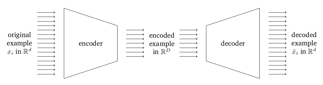
We want to train in such a way as to minimize the distance between the original examples in $\R^d$ and the "recovered" examples that result from encoding and then decoding the example. Formally, given some dataset $x_1, \ldots, x_n$, we want to minimize
$$\frac{1}{n} \sum_{i=1}^n \norm{ \psi(\phi(x_i)) - x_i }^2$$over some parameterized class of nonlinear transformations $\phi: \R^d \rightarrow \R^r$ and $\psi: \R^r \rightarrow \R^d$ defined by a neural network.
Sparsity
An alternate approach to deal with large dimension $d$ is sparsity.
A vector or matrix is informally called sparse when few of its entries are non-zero.
The density of a sparse matrix or vector is the fraction of its entries that are non-zero. For example, the vector
has density $3/10 = 0.3$.
When the density of a matrix is low, we can store and compute with it in a format specialized for sparse matrices.
This results in computations that have cost proportional to the number of nonzero entries of the matrix, rather than its dimensions.
- So if $d$ is large, but the matrices involved have low density, we can often save a lot of compute and memory by using sparse matrix formats.
Storing sparse vectors.
The standard way to store a sparse vector to store only the nonzero entries as pairs consisting of the index and the value of the nonzero entry.
Concretely, for the vector above, we would store it as
$$(\texttt{index: } 0, \texttt{value: } 3), (\texttt{index: } 4, \texttt{value: } 2), (\texttt{index: } 8, \texttt{value: } 7).$$Usually this is stored more compactly as two arrays: one array of indexes and one array of values.
\begin{align*} \texttt{indexes: } & \begin{bmatrix} 0 & 4 & 8 \end{bmatrix} \\ \texttt{values: } & \begin{bmatrix} 3 & 2 & 7 \end{bmatrix}. \end{align*}Storing sparse matrices.
There are many ways to store a sparse matrix. The simplest way is a direct adaptation of the way to store sparse vectors: we store the indexes (as a row/column pair) and values of all the nonzero entries. This format is called "coordinate list" or COO. For example, the matrix
$$\begin{bmatrix} 5 & 0 & 0 & 3 & 0 & 1 \\ 0 & 4 & 0 & 0 & 0 & 0 \\ 1 & 2 & 0 & 0 & 3 & 0 \end{bmatrix}$$could be encoded in COO as
\begin{align*} \texttt{row indexes: } & \begin{bmatrix} 0 & 0 & 0 & 1 & 2 & 2 & 2 \end{bmatrix} \\ \texttt{column indexes: } & \begin{bmatrix} 0 & 3 & 5 & 1 & 0 & 1 & 4 \end{bmatrix} \\ \texttt{values: } & \begin{bmatrix} 5 & 3 & 1 & 4 & 1 & 2 & 3 \end{bmatrix}. \end{align*}Note that for COO, the order of the nonzero entries does not matter and no particular order is specified, although they are often sorted for performance reasons.
Storing Sparse Matrices Continued
Another common format is "compressed sparse row" or CSR. CSR effectively stores all the rows of the matrix as sparse vectors concatenated into one big array, and then uses another row offset array to index into it. The above matrix encoded in CSR would look like
\begin{align*} \texttt{row offsets: } & \begin{bmatrix} 0 & 3 & 4 \end{bmatrix} \\ \texttt{column indexes: } & \begin{bmatrix} 0 & 3 & 5 & 1 & 0 & 1 & 4 \end{bmatrix} \\ \texttt{values: } & \begin{bmatrix} 5 & 3 & 1 & 4 & 1 & 2 & 3 \end{bmatrix} \end{align*}where $0$, $3$, and $4$ are the offsets within the column index and values arrays at which rows $0$, $1$, and $2$ begin, respectively.
"Compressed sparse column," or CSC is just the transpose-dual of CSR: it stores the columns of a matrix as sparse vectors rather than the rows.
Comparing Storage Formats
While COO is better for building matrices by adding entries, CSR usually allows for faster matrix multiply with dense vectors and matrices.
Sparsity Epilogue: Other storage formats.
There are many other ways to store sparse matrices, especially in the case where the matrix has some structure
- for example, if it is banded matrix or a symmetric matrix
- or a tridiagonal matrix
Some sparse matrix formats take advantage of dense sub-blocks within the matrix, which they store in a dense format to save memory and compute.