Data Assumption: \(y_{i} \in \mathbb{R}\)
Model Assumption: \(y_{i} = \mathbf{w}^\top\mathbf{x}_i +
\epsilon_i\) where \(\epsilon_i \sim N(0, \sigma^2)\)
\(\Rightarrow y_i|\mathbf{x}_i \sim N(\mathbf{w}^\top\mathbf{x}_i, \sigma^2)
\Rightarrow
P(y_i|\mathbf{x}_i,\mathbf{w})=\frac{1}{\sqrt{2\pi\sigma^2}}e^{-\frac{(\mathbf{x}_i^\top\mathbf{w}-y_i)^2}{2\sigma^2}}\)
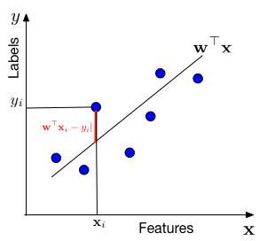
In words, we assume that the data is drawn from a "line" \(\mathbf{w}^\top
\mathbf{x}\) through the origin (one can always add a bias / offset
through an additional dimension, similar to the
Perceptron). For each data point with
features \(\mathbf{x}_i\), the label \(y\) is drawn from a Gaussian with
mean \(\mathbf{w}^\top \mathbf{x}_i\) and variance \(\sigma^2\). Our task
is to estimate the slope \(\mathbf{w}\) from the data.
Estimating with MLE
\[ \begin{aligned} \mathbf{w} &= \operatorname*{argmax}_{\mathbf{\mathbf{w}}} P(D|\mathbf{w}) &\textrm{Definition of MLE;}\\
&=
\operatorname*{argmax}_{\mathbf{\mathbf{w}}}
P(y_1,\mathbf{x}_1,...,y_n,\mathbf{x}_n|\mathbf{w})&\textrm{Unpacking $D$;}\\
&=
\operatorname*{argmax}_{\mathbf{\mathbf{w}}} \prod_{i=1}^n
P(y_i,\mathbf{x}_i|\mathbf{w}) & \textrm{Because data points are
independently sampled.}\\ &=
\operatorname*{argmax}_{\mathbf{\mathbf{w}}} \prod_{i=1}^n
P(y_i|\mathbf{x}_i,\mathbf{w})P(\mathbf{x}_i|\mathbf{w}) &
\textrm{Chain rule of probability.}\\ &=
\operatorname*{argmax}_{\mathbf{\mathbf{w}}} \prod_{i=1}^n
P(y_i|\mathbf{x}_i,\mathbf{w})P(\mathbf{x}_i) &
\textrm{\(\mathbf{x}_i\) is independent of \(\mathbf{w}\), we only model
\(P(y_i|\mathbf{x})\)}\\ &=
\operatorname*{argmax}_{\mathbf{\mathbf{w}}} \prod_{i=1}^n
P(y_i|\mathbf{x}_i,\mathbf{w}) & \textrm{\(P(\mathbf{x}_i)\) is a
constant - can be dropped}\\ &=
\operatorname*{argmax}_{\mathbf{\mathbf{w}}} \sum_{i=1}^n
\log\left[P(y_i|\mathbf{x}_i,\mathbf{w})\right] & \textrm{log is a
monotonic function}\\ &= \operatorname*{argmax}_{\mathbf{\mathbf{w}}}
\sum_{i=1}^n \left[ \log\left(\frac{1}{\sqrt{2\pi\sigma^2}}\right) +
\log\left(e^{-\frac{(\mathbf{x}_i^\top\mathbf{w}-y_i)^2}{2\sigma^2}}\right)\right]
& \textrm{Plugging in probability distribution}\\ &=
\operatorname*{argmax}_{\mathbf{\mathbf{w}}}
-\frac{1}{2\sigma^2}\sum_{i=1}^n (\mathbf{x}_i^\top\mathbf{w}-y_i)^2 &
\textrm{First term is a constant, and \(\log(e^z)=z\)}\\ &=
\operatorname*{argmin}_{\mathbf{\mathbf{w}}} \frac{1}{n}\sum_{i=1}^n
(\mathbf{x}_i^\top\mathbf{w}-y_i)^2 &
\textrm{Always minimize;
\(\frac{1}{n}\) makes loss interpretable (avg. squared error).}\\
\end{aligned} \]
We are minimizing a loss function, \(l(\mathbf{w}) =
\frac{1}{n}\sum_{i=1}^n (\mathbf{x}_i^\top\mathbf{w}-y_i)^2\). This
particular loss function is also known as the squared loss. Linear regression is also known as Ordinary
Least Squares (OLS). OLS can be optimized with gradient descent or Newton's method. The latter leads to a closed-form solution.
Closed Form: \(\mathbf{w} = (\mathbf{X
X^\top})^{-1}\mathbf{X}\mathbf{y}^\top\) where
\(\mathbf{X}=\left[\mathbf{x}_1,\dots,\mathbf{x}_n\right]\) and
\(\mathbf{y}=\left[y_1,\dots,y_n\right]\).
This objective is known as Ridge Regression. It has a closed form solution
of: \(\mathbf{w} = (\mathbf{X X^{\top}}+\lambda
\mathbf{I})^{-1}\mathbf{X}\mathbf{y}^\top,\) where
\(\mathbf{X}=\left[\mathbf{x}_1,\dots,\mathbf{x}_n\right]\) and
\(\mathbf{y}=\left[y_1,\dots,y_n\right]\).
 Data Assumption: \(y_{i} \in \mathbb{R}\)