Goal: We want to minimize a convex, continuous and differentiable loss function \(\ell(w)\). In this section we discuss two of the most popular "hill-climbing" algorithms, gradient descent and Newton's method.
General form for the algorithm:How can you minimize a function \(\ell\) if you don't know much about it? The trick is to assume it is much simpler than it really is. This can be done with Taylor's approximation.
Taylor's Theorem (Lagrange form). Let \( k \ge 1 \) be a natural number, \(x \in \mathbb{R}\), and \( f: \mathbb{R} \rightarrow \mathbb{R} \) be a function that is \((k+1)\)-times continuously differentiable on \( [0, x] \). Then there exists some \( \zeta \in [0, x] \) such that \[ f(x) = f(0) + x f'(0) + \frac{x^2}{2} f''(0) + \cdots + \frac{x^k}{k!} f^{(k)}(0) + \frac{x^{k+1}}{(k+1)!} f^{(k+1)}(\zeta). \]
As direct consequence of Taylor's theorem, we have the following result for multidimensional functions. If \( \ell: \mathbb{R}^d \rightarrow \mathbb{R} \) is continuously twice differentiable, then for any \( w \in \mathbb{R}^d \) and any \( s \in \mathbb{R}^d \), there exists a \( \zeta \in [0,1] \) such that \[ \ell(w + s) = \ell(w) + s^T \nabla \ell(w) + \frac{1}{2} s^T \nabla^2 \ell(w + \zeta s) s = \ell(w) + s^T \nabla \ell(w) + \mathcal{O}(\| s \|^2), \] where \( \nabla \ell(w) \in \mathbb{R}^d \) is the gradient of \( \ell \) and \( \nabla^2 \ell(w) \in \mathbb{R}^{d \times d} \) is its second-derivative matrix, a.k.a. its Hessian matrix. Similarly, if \( \ell: \mathbb{R}^d \rightarrow \mathbb{R} \) is continuously thrice differentiable, then \[ \ell(w + s) = \ell(w) + s^T \nabla \ell(w) + \frac{1}{2} s^T \nabla^2 \ell(w) s + \mathcal{O}(\| s \|^3). \]
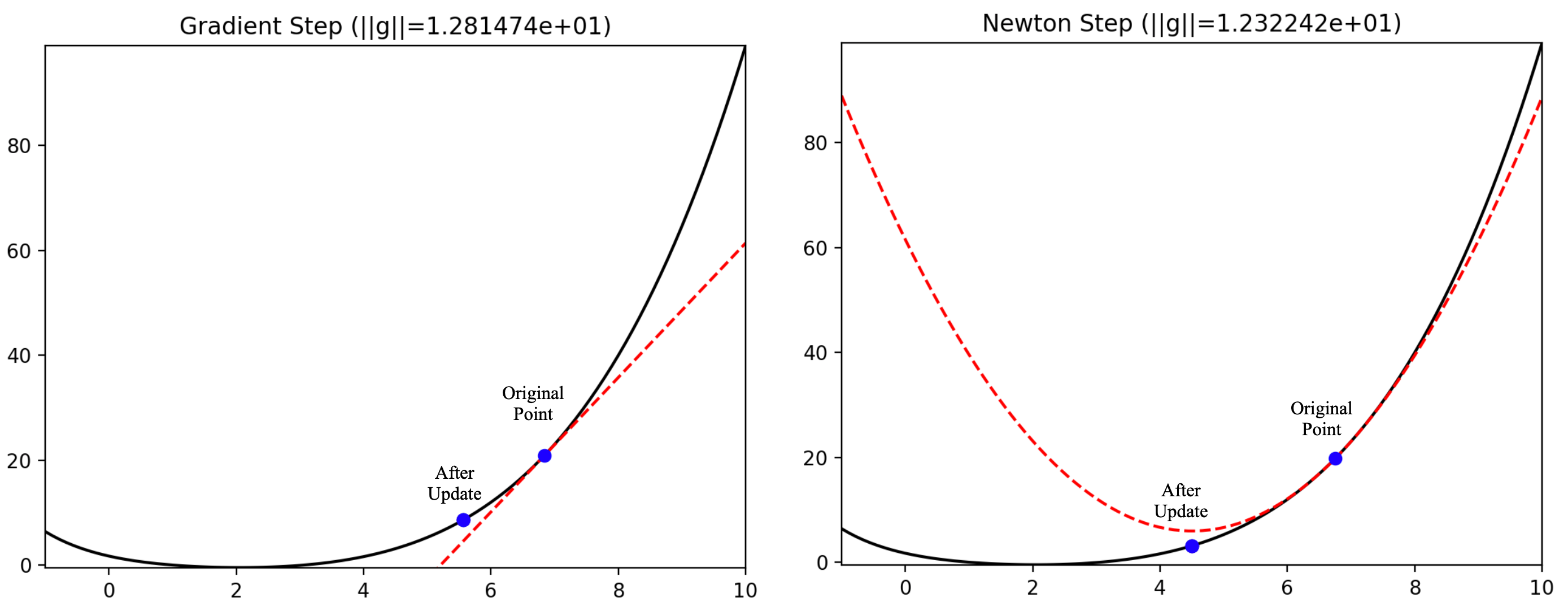
So, provided that the norm \(\|s\|_2\) is small (i.e. \({w}\) + \(s\) is very close to \({w}\)), we can approximate the function \(\ell({w} + s)\) by its first and second derivatives: \[ \ell(w + s) \approx \ell(w) + s^T \nabla \ell(w), \] \[ \ell(w + s) \approx \ell(w) + s^T \nabla \ell(w) + \frac{1}{2} s^T \nabla^2 \ell(w) s. \] Both approximations are valid if \(\|s\|_2\) is small, but the second one assumes that \(\ell\) is twice differentiable (at least, and thrice differentiable if we want the error term to be \( \mathcal{O}(\| s \|^3) \) ) and is more expensive to compute but also more accurate than only using gradient.In gradient descent we only use the gradient (first order). In gradient descent we simply set \[ s = -\alpha \nabla \ell(w), \] for some small scalar \(\alpha > 0 \) called the "step size" or "learning rate." It is straight-forward to prove that for sufficiently small \(\alpha\), \(\ell({w}+s) \le \ell({w})\). For some \( \zeta \in [0,1] \), if the Hessian of \( \ell \) is bounded everywhere, then \begin{align*} \ell(w - \alpha \nabla \ell(w)) &= \ell(w) + \left( - \alpha \nabla \ell(w) \right)^T \nabla \ell(w) \\&\hspace{2em}+ \frac{1}{2} \left( - \alpha \nabla \ell(w) \right)^T \nabla^2 \ell(w - \zeta \alpha \nabla \ell(w)) \left( - \alpha \nabla \ell(w) \right) \\&= \ell(w) - \alpha \| \nabla \ell(w) \|^2 + \frac{\alpha^2}{2} \nabla \ell(w)^T \nabla^2 \ell(w - \zeta \alpha \nabla \ell(w)) \nabla \ell(w), \\&= \ell(w) - \alpha \| \nabla \ell(w) \|^2 + \| \nabla \ell(w) \|^2 \mathcal{O}(\alpha^2). \end{align*} Of course \( -\alpha + \mathcal{O}(\alpha^2) \) is guaranteed to be negative for sufficiently small step sizes \( \alpha \). In particular, there must be an \(\alpha\) small enough that \( \ell(w - \alpha \nabla \ell(w)) \le \ell(w) - \frac{\alpha}{2} \| \nabla \ell(w) \|^2 \).
Just like we did for the perceptron, we can show that gradient descent converges: that is, that no matter what threshold \( \delta \) we pick to stop at, our steps \( s_t \) will eventually have \( \| s_t \| \le \delta \). Here I'll outline a proof that if converges under the really simple assumptions that (1) \( \ell \) is non-negative, i.e. \( \ell(w) \ge 0 \), and (2) we choose a fixed \(\alpha\) small enough that \( \ell(w - \alpha \nabla \ell(w)) \le \ell(w) - \frac{\alpha}{2} \| \nabla \ell(w) \|^2 \). (We can also prove gradient descent converges in a variety of other ways under different assumptions: there are whole courses on this sort of thing.)
Recall that \(w_t \in \mathbb{R}^d \) denotes the state of gradient descent after \(t\) iterations. By our assumption that the step size is sufficiently small, we'll have that \[ \ell(w_{t+1}) \le \ell(w_t) - \frac{\alpha}{2} \| \nabla \ell(w_t) \|^2 = \ell(w_t) - \frac{1}{2 \alpha} \| s_t \|^2, \] since \( s_t = - \alpha \nabla \ell(w_t) \). Now, if we have not converged at step \(t\), then ipso facto \( \| s_t \| > \delta \) and so \[ \ell(w_{t+1}) \le \ell(w_t) - \frac{\delta^2}{2 \alpha}. \] That is, at each step the loss must decrease by at least \( \delta^2 / 2 \alpha \). But this can't continue indefinitely! Applying this inductively over \(T\) total steps, we must have that \[ \ell(w_T) \le \ell(w_0) - \frac{\delta^2 T}{2 \alpha}. \] Using our assumption that \(\ell \) is non-negative, \[ 0 \le \ell(w_T) \le \ell(w_0) - \frac{\delta^2 T}{2 \alpha}, \] and solving for \(T\) gives \[ T \le \frac{2 \alpha \ell(w_0)}{\delta^2}. \] This shows that gradient descent must terminate eventually!
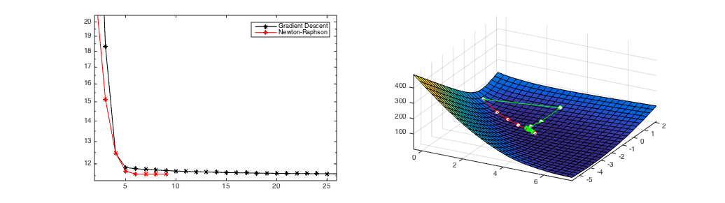
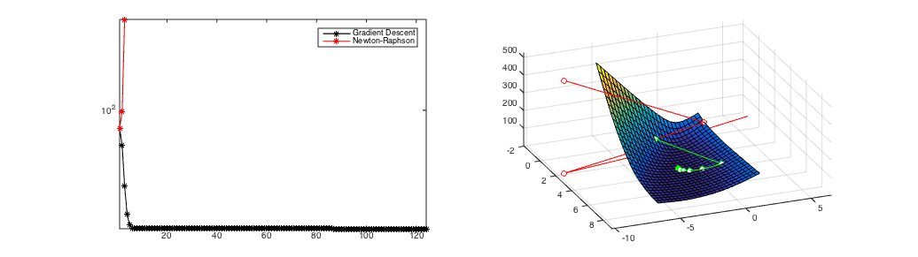
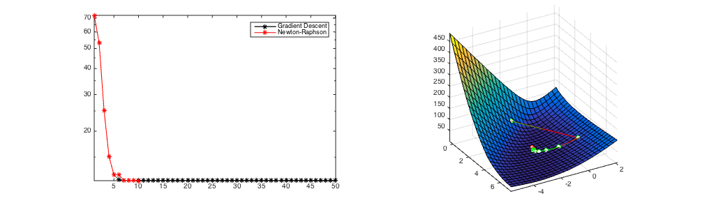
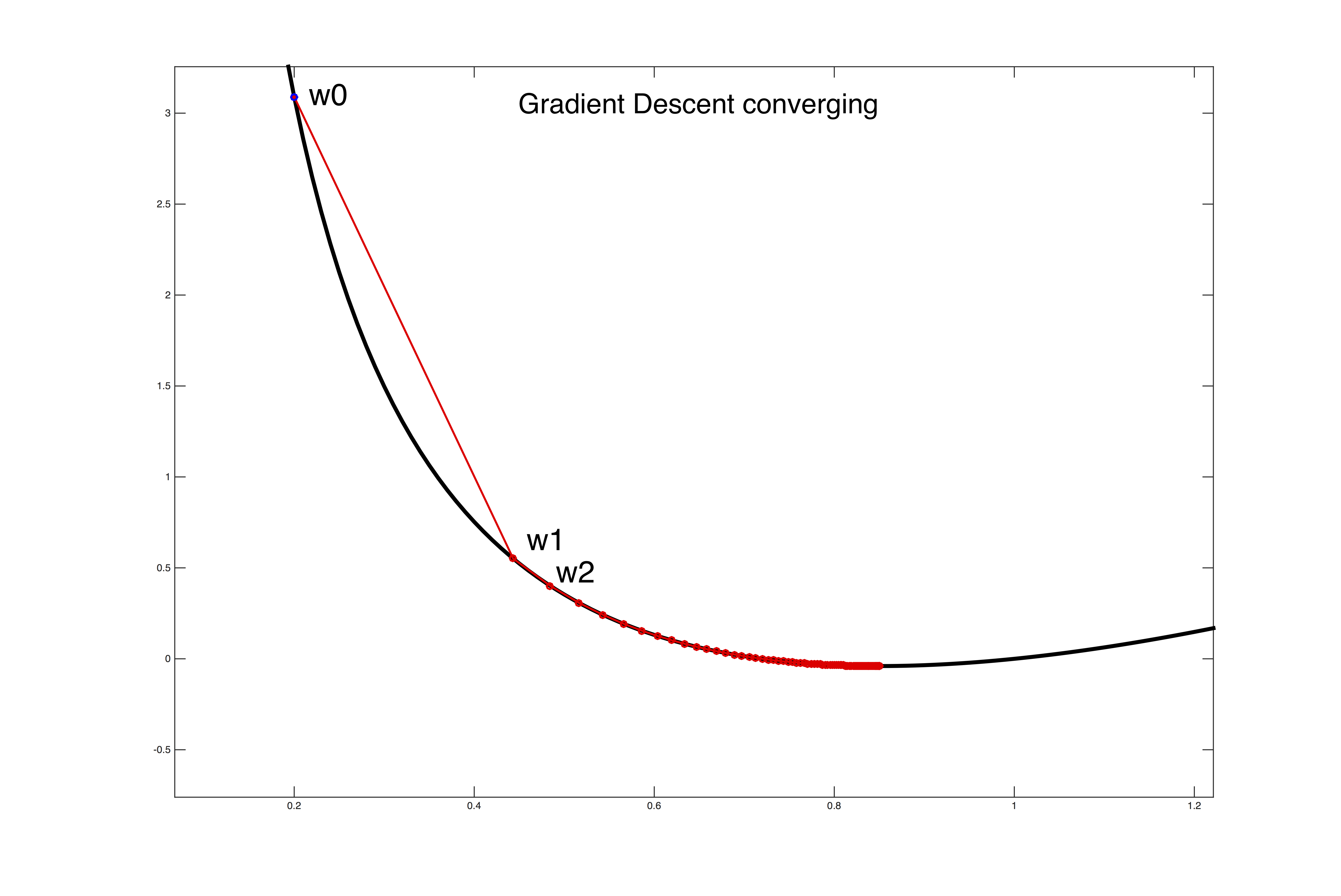
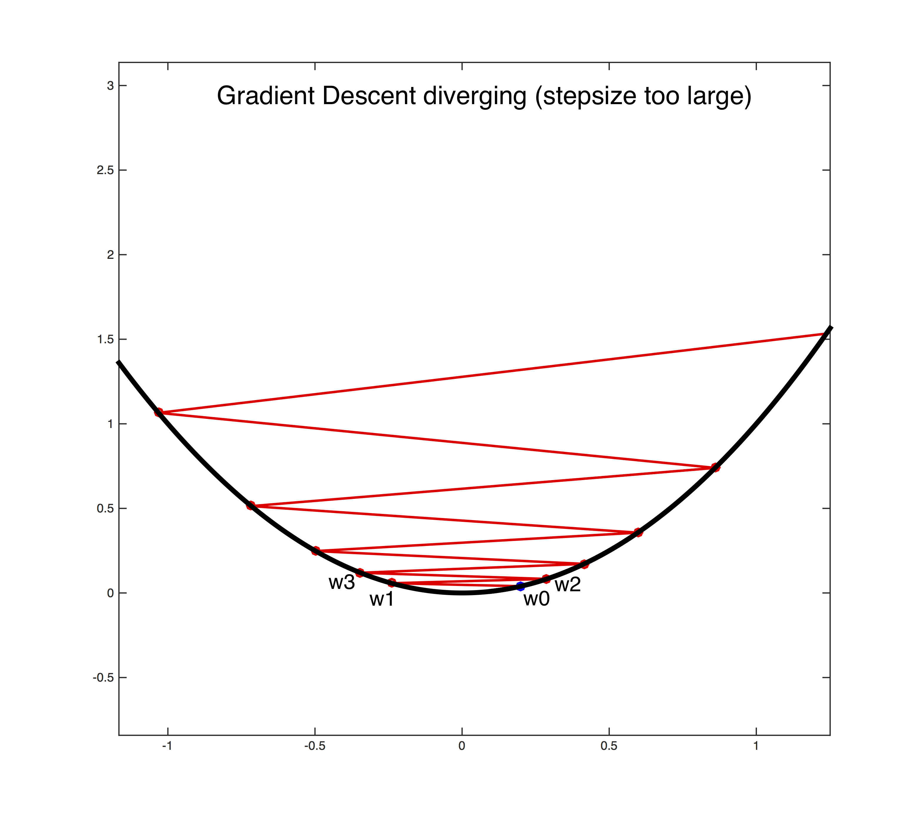
Setting the learning rate \(\alpha > 0 \) is a dark art. Only if it is sufficiently small will gradient descent converge (see the first figure below). If it is too large the algorithm can easily diverge out of control (see the second figure below). But on the other hand, if it's too small, then GD may make a small step (and so decide to stop since \( \| s \| \le \delta \)) while still far from the optimum, and generally with smaller step sizes GD takes longer to converge to the same value of the loss. A safe (but sometimes slow) choice is to use a diminishing step size scheme \(\alpha_t = \frac{\alpha_0}{t + 1}\), which guarantees that it will eventually become small enough to converge (for any initial value \(\alpha_0 \ge 0 \).
One option is to set the step-size adaptively for every feature. Adagrad keeps a running average of the squared gradient magnitude and sets a small learning rate for features that have large gradients, and a large learning rate for features with small gradients. Setting different learning rates for different features is particularly important if they are of different scale or vary in frequency. For example, word counts can differ a lot across common words and rare words.
Adagrad Algorithm:
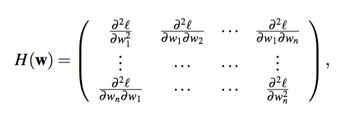
Newton's method assumes that the loss \(\ell\) is twice differentiable and uses the approximation with Hessian (2nd order Taylor approximation). The Hessian Matrix \( H(w) = \nabla^2 \ell(w) \) contains all second order partial derivatives and is defined as
Note: A symmetric matrix \( M \in \mathbb{R}^{d \times d} \) is positive semi-definite if it has only non-negative eigenvalues or, equivalently, for any vector \( x \in \mathbb{R}^d \) we must have \( x^T M x \ge 0\).
It follows that the approximation \[ \ell(w + s) \approx \ell(w) + s^T \nabla \ell(w) + \frac{1}{2} s^T H(w) s \] describes a convex parabola, and we can find its minimum by solving the following optimization problem: \[ \arg \min_{s \in \mathbb{R}^d} \; \ell(w) + s^T \nabla \ell(w) + \frac{1}{2} s^T H(w) s. \] To find the minimum of the objective, we take its first derivative with respect to \(s\), equate it with zero, and solve for \(s\): \begin{align} g({w}) + H({w})s&=0\\ \Rightarrow s&= -(H({w}))^{-1}g({w}). \end{align} This results in the update step \[ w_{t+1} = w_t - (H({w_t}))^{-1}g({w_t}). \]
This choice of \(s\) converges extremely fast if the approximation is sufficiently accurate and the resulting step sufficiently small. Otherwise it can diverge. Divergence often happens if the function is flat or almost flat with respect to some dimension. In that case the second derivatives are close to zero, and their inverse becomes very large—resulting in gigantic steps. Different from gradient descent, here there is no step-size that guarantees that steps are all small and local. As the Taylor approximation is only accurate locally, large steps can move the current estimates far from regions where the Taylor approximation is accurate.