Learning by Maximizing Probability

Cornell CS 4/5780

Spring 2022

Old Recorded Lectures

Motivation

Recall the Bayes Optimal classifier. If we are provided with the true source distribution $ \mathcal{P} $ over example-label pairs $ (X, Y) $, we can predict the most likely label for $\mathbf{x}$: $\operatorname*{argmax}_y \mathcal{P}(y|\mathbf{x}). $ One very general approach to learning motivated by this is to estimate $ \mathcal{P} $ directly from the training data. If it is possible (to a good approximation) to construct an estimate $ \hat{\mathcal{P}} \approx \mathcal{P} $ we could then use the Bayes Optimal classifier on $ \hat{\mathcal{P}} $ in practice.

Many supervised learning strategies can be viewed as estimating $ \mathcal{P} $. Generally, they fall into two categories:

When we estimate the full joint distribution $\mathbf{P}(X,Y)=\mathbf{P}(X|Y)\mathbf{P}(Y)$, then we call it generative learning, named after the fact that we can use the estimate of $ \mathcal{P} $ to generate new samples that approximate the source distribution.
When we only estimate the conditional distributions $\mathbf{P}(Y|X)$ directly, then we call it discriminative learning.

So how can we estimate probability distributions from samples?

Simple scenario: coin toss

Suppose you find a coin and it's ancient and very valuable. Naturally, you ask yourself, "What is the probability that this coin comes up heads when I toss it?" You toss it $n = 10$ times and obtain the following (ordered) sequence of outcomes: $D=\{H, T, T, H, H, H, T, T, T, T\}$. Based on these samples, how would you estimate $P(H)$? We observed $n_H=4$ heads and $n_T=6$ tails. So, intuitively, $$ P(H) \approx \frac{n_H}{n_H + n_T} = \frac{4}{10}= 0.4. $$ But is this reasoning valid? Can we derive this more formally?

Maximum Likelihood Estimation (MLE)

The estimator we just mentioned is the Maximum Likelihood Estimate (MLE). For MLE you typically proceed in two steps.

First, you make an explicit modeling assumption about what type of distribution your data was sampled from.
Second, you set the parameters of this distribution so that the data you observed is as likely as possible.

Let us return to the coin example. A natural assumption about a sequence of coin tosses (for a particular coin with a fixed probability of coming up heads) is that the results of the flips are independent. Formally, if $ X_i \in \{0,1\} $ is the indicator random variable representing the event that the result of the $i$th flip is heads, and we suppose that the probability of the coin coming up heads is $ \theta \in [0,1] $, then \[ \mathbf{P}(X_i = x_i; \theta) = \begin{cases} \theta & \text{ if } x_i = 1 \\ 1 - \theta & \text{ if } x_i = 0 \end{cases} = \theta^{x_i} (1 - \theta)^{1 - x_i}. \] By independence, the probability of many such flips coming up in any particular way (i.e. in some specific order $ x_1, x_2, \ldots, x_n $) will be the product of the probabilities \begin{align*} \mathbf{P}(X_1 = x_1, X_2 = x_2, \ldots, X_n = x_n; \theta) &= \prod_{i=1}^n \mathbf{P}(X_i = x_i; \theta) \\&= \prod_{i=1}^n \theta^{x_i} (1 - \theta)^{1 - x_i} \\&= \theta^{\sum_{i=1}^n x_i} (1 - \theta)^{\sum_{i=1}^n (1 - x_i)}. \end{align*} We can write this a little more consisely if we let $ n_H = \sum_{i=1}^n x_i $ denote the number of heads and $ n_T = \sum_{i=1}^n 1 - x_i $ denote the number of tails. In this case, we would just have \[ \mathbf{P}(X_1 = x_1, X_2 = x_2, \ldots, X_n = x_n; \theta) = \theta^{n_H} (1 - \theta)^{n_T}. \]

MLE Principle: Find $\hat{\theta}$ to maximize the likelihood of the data, $ \mathbf{P}(\mathcal{D}; \theta)$: \begin{align} \hat{\theta}_{MLE} &= \operatorname*{argmax}_{\theta} \, \mathbf{P}( \mathcal{D} ; \theta), \end{align} where here we slightly abuse notation to let $ \mathcal{D} $ also denote the event that the dataset $ \mathcal{D} $ is observed.

Often we can solve this maximization problem with a simple three step procedure:

Plug in all the terms for the distribution, and take the $\log$ of the function.
Compute its derivative, and equate it with zero.
Solve the resulting equation for $ \theta $, and check that it's a maximum.

Taking the log of the likelihood (often referred to as the log-likelihood) does not change its maximum (as the log is a monotonic function, and the likelihood positive), but it turns all products into sums which are much easier to deal with when you differentiate. Equating the derivative with zero is a standard way to find an extreme point. (To be precise you should verify that it really is a maximum and not a minimum or a saddle point, by verifying that the Hessian is negative-definite.)

Returning to our coin-flipping example, we can now plug in the definition and compute the log-likelihood: \begin{align} \hat{\theta}_{\operatorname{MLE}} &= \operatorname*{argmax}_{\theta} \; \mathbf{P}(D; \theta) \\ &= \operatorname*{argmax}_{\theta} \; \theta^{n_H} (1 - \theta)^{n_T} \\ &= \operatorname*{argmax}_{\theta} \; \log\left( \theta^{n_H} (1 - \theta)^{n_T} \right) \\ &= \operatorname*{argmax}_{\theta} \; n_H \cdot \log(\theta) + n_T \cdot \log(1 - \theta). \end{align} We can then solve for $\theta$ by taking the derivative and equating it with zero. This results in \begin{align} 0 = \frac{n_H}{\theta} - \frac{n_T}{1 - \theta} \Longrightarrow n_H - n_H\theta = n_T\theta \Longrightarrow \theta = \frac{n_H}{n_H + n_T}. \end{align} A nice sanity check is that $\theta\in[0,1]$.

MLE gives the explanation of the data you observed.
If your model/distribution family includes the true source distribution — that is, there exists some $ \theta $ such that $ \mathcal{P}(x,y) = \mathbf{P}(X = x, Y = y; \theta) $ — then as the number of independent examples $ n $ approaches infinity, the distribution produced by MLE approaches the true source distribution $ \mathcal{P} $.
But the MLE can overfit the data if $n$ is small. It works well when $n$ is large.
If you do not have the correct model then MLE can be terribly wrong!

For example, suppose you observe H,H,H,H,H. What is $\hat{\theta}_{MLE}$?

Simple scenario: coin toss with prior knowledge

Suppose you have a hunch that $\theta$ is close to $ \frac{1}{2} $. But your sample size is small, so you don't trust your estimate. Simple fix: Add $m$ imaginary throws that would result in the $\theta$ we have a hunch it is close to (e.g. $\theta = 0.5$). For example, we could add $m$ Heads and $m$ Tails to your data, which would result in the modified MLE estimate $$ \hat{\theta} = \frac{n_H + m}{n_H + n_T + 2m} $$ For large $n$, this is an insignificant change. For small $n$, it incorporates your "prior belief" about what $\theta$ should be. But this was all very ad hoc. Can we justify this and derive it formally?

The Bayesian Way

Model $\theta$ as a random variable, with its own marginal distribution $ \mathbf{P}(\theta)$. Here $ \theta $ and the other observed variables $ (x_i, y_i) $ are jointly distributed.

Note that $\theta$ is not a random variable associated with an event in a sample space. In frequentist statistics, this is forbidden. In Bayesian statistics, this is allowed and you can specify a prior belief $\mathbf{P}(\theta)$ defining what values you believe $\theta$ is likely to take on.

Now, we can look at $ \mathbf{P}(\theta \mid \mathcal{D} ) = \frac{ \mathbf{P}(\mathcal{D} \mid \theta) \mathbf{P}(\theta)}{ \mathbf{P}(\mathcal{D} )}$ (recall Bayes Rule!), where

$ \mathbf{P}(\theta)$ is the prior distribution over the parameter(s) $\theta$, before we see any data.
$ \mathbf{P}(\mathcal{D} \mid \theta)$ is the likelihood of the data given the parameter(s) $\theta$.
$ \mathbf{P}(\theta \mid \mathcal{D})$ is the posterior distribution over the parameter(s) $\theta$ after we have observed the data.

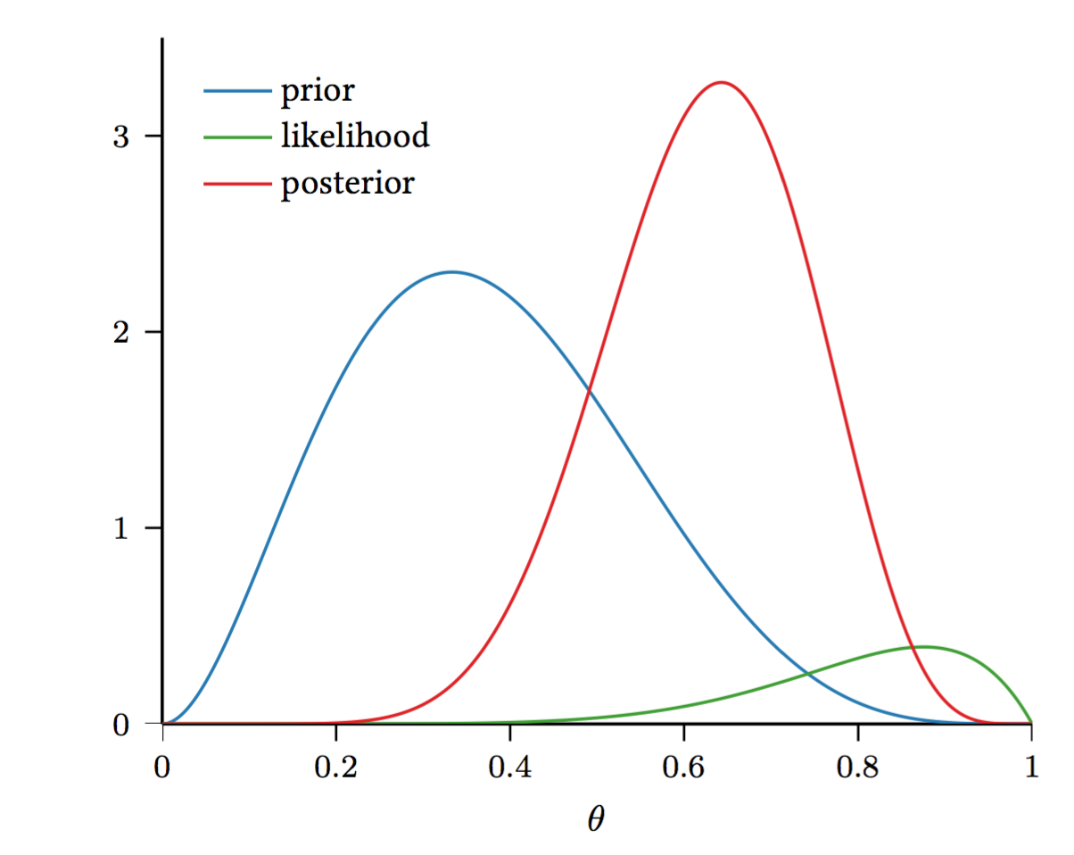
A natural choice for the prior $\mathbf{P}(\theta$) is the Beta distribution: \begin{align} \mathbf{P}(\theta) = \frac{\theta^{\alpha - 1}(1 - \theta)^{\beta - 1}}{B(\alpha, \beta)} \end{align} where the beta function \[ B(\alpha, \beta) = \frac{\Gamma(\alpha) \Gamma(\beta)}{\Gamma(\alpha+\beta)} = \int_{0}^{1} \theta^{\alpha - 1} (1 - \theta)^{\beta - 1} \; d \theta \] is the normalization constant (if this looks scary don't worry about it, it is just there to make sure everything sums to $1$ and to scare children at Halloween). Note that here we only need a distribution over a single random variable $\theta$. (The multivariate generalization of the Beta distribution is the Dirichlet distribution.)

Why is the Beta distribution a good fit?

it models probabilities ($\theta$ lives on $\left[0,1\right]$)
it is the conjugate prior of (the same distributional family as) the binomial distribution, which is the distribution of the number of heads that would come up in this experiment. This means that the math will turn out nicely:

\begin{align} \mathbf{P}(\theta \mid \mathcal{D}) \propto \mathbf{P}(\mathcal{D} \mid \theta) \mathbf{P}(\theta) \propto \theta^{n_H + \alpha - 1} (1 - \theta)^{n_T + \beta - 1}. \end{align}

So far, we have a distribution over $\theta$. How can we get an estimate for $\theta$?

Maximum a Posteriori Probability Estimation (MAP)

MAP Principle: Find $\hat{\theta}$ that maximizes the posterior distribution $ \mathbf{P}(\theta \mid \mathcal{D})$: \begin{align} \hat{\theta}_{\operatorname{MAP}} &= \operatorname*{argmax}_{\theta} \; \mathbf{P}(\theta \mid \mathcal{D}) \\ &= \operatorname*{argmax}_{\theta} \; \frac{ \mathbf{P}(\mathcal{D} \mid \theta) \mathbf{P}(\theta) }{ \mathbf{P}(\mathcal{D}) } && \text{(by Bayes rule)} \\ &= \operatorname*{argmax}_{\theta} \; \mathbf{P}(\mathcal{D} \mid \theta) \mathbf{P}(\theta) && \text{(drop constant factor)} \\ &= \operatorname*{argmax}_{\theta} \; \log \mathbf{P}(\mathcal{D} \mid \theta) + \log \mathbf{P}(\theta) && \text{(take log)} \end{align} For out coin flipping scenario, we get: \begin{align} \hat{\theta}_{\operatorname{MAP}} &= \operatorname*{argmax}_{\theta} \; \log \mathbf{P}(\mathcal{D} \mid \theta) + \log \mathbf{P}(\theta) \\ &= \operatorname*{argmax}_{\theta} \;n_H \cdot \log(\theta) + n_T \cdot \log(1 - \theta) \\&\hspace{8em}+ (\alpha - 1)\cdot \log(\theta) + (\beta - 1) \cdot \log(1 - \theta) - \log(B(\alpha,\beta)) \\ &= \operatorname*{argmax}_{\theta} \;(n_H + \alpha - 1) \cdot \log(\theta) + (n_T + \beta - 1) \cdot \log(1 - \theta) \\ \Longrightarrow \hat{\theta}_{MAP} &= \frac{n_H + \alpha - 1}{n_H + n_T + \beta + \alpha - 2} \end{align}

A few comments:

The MAP estimate is identical to MLE with $\alpha-1$ hallucinated heads and $\beta-1$ hallucinated tails. (At least, if $\alpha$ and $\beta$ are integers.)
As $n \rightarrow \infty$, $\hat\theta_{MAP} \rightarrow \hat\theta_{MLE}$ as $\alpha-1$ and $\beta-1$ become irrelevant compared to very large $n_H,n_T$.
MAP is a great estimator if an accurate prior belief is available (and mathematically tractable).
If $n$ is small, MAP can be very wrong if prior belief is wrong!

The "True" Bayesian approach

MAP is only one way to get an estimator. There is much more information in $ \mathbf{P}(\theta \mid \mathcal{D})$, and it seems like a shame to simply compute the mode and throw away all other information. A true Bayesian approach is to use the posterior predictive distribution directly to make predictions about the label $Y$ of a test sample with features $X$. Here we consider $X$ and $Y$ to be a "fresh" test example independent of all the examples in the training dataset conditioned on $ \theta $. Concretely, this corresponds to the distribution over $ y $ given by \begin{align*} \hat{\mathcal{P}}(x, y) = \int \mathbf{P}(Y = y \mid X = x, \theta = \vartheta) \mathbf{P}(\theta = \vartheta | \mathcal{D} ) \; d\vartheta. \end{align*} Unfortunately, the above is generally intractable in closed form. Sampling techniques, such as Monte Carlo approximations, are used to approximate the distribution. A common exception where this is tractable is the case of Gaussian Processes.

Another exception is actually our coin toss example. Here, we don't really have features, so we can ignore the $ X $ in the above formulation. To make predictions using $\theta$ in our coin tossing example, we can see that the distribution of a fresh flip is \begin{align} \hat{\mathcal{P}}(y) =& \int_0^1 \mathbf{P}(Y = y \mid \theta = \vartheta) \mathbf{P}(\theta = \vartheta | \mathcal{D} ) \; d\vartheta \\ =& \int_0^1 \mathbf{P}(Y = y \mid \theta = \vartheta) \cdot \frac{ \mathbf{P}(\mathcal{D} \mid \theta = \vartheta ) \mathbf{P}(\theta = \vartheta )}{\mathbf{P}( \mathcal{D} )} \; d\vartheta \\ =& \int_0^1 \vartheta^{y} (1 - \vartheta)^{1 - y} \cdot \frac{ \vartheta^{n_H + \alpha - 1} (1 - \vartheta)^{n_T + \beta - 1} }{B(\alpha, \beta) \cdot \mathbf{P}( \mathcal{D} )} \; d\vartheta. \end{align} If we let $ Z = B(\alpha, \beta) \mathbf{P}(\mathcal{D}) $, which is just a constant independent of $ y $, then \begin{align} \hat{\mathcal{P}}(1) =& \frac{1}{Z} \int_0^1 \vartheta^{n_H + \alpha} (1 - \vartheta)^{n_T + \beta - 1} \; d\vartheta \end{align} and \begin{align} \hat{\mathcal{P}}(0) =& \frac{1}{Z} \int_0^1 \vartheta^{n_H + \alpha - 1} (1 - \vartheta)^{n_T + \beta} \; d\vartheta. \end{align} Integrating the former by parts (and observing that the boundary term is $0$ because it vanishes at both $0$ and $1$) gives \begin{align} \hat{\mathcal{P}}(1) =& \frac{1}{Z} \int_0^1 \left( n_H + \alpha \right)\vartheta^{n_H + \alpha - 1} \cdot \frac{1}{n_T + \beta} (1 - \vartheta)^{n_T + \beta} \; d\vartheta \\=& \frac{n_H + \alpha}{n_T + \beta} \hat{\mathcal{P}}(0) \\=& \frac{n_H + \alpha}{n_T + \beta} \left( 1 - \hat{\mathcal{P}}(1)\right), \end{align} and so \[ \hat{\mathcal{P}}(1) = \frac{n_H + \alpha}{n_H + n_T + \alpha + \beta}. \] Effectively, this says that the Bayesian posterior for a fresh example drawn from the distribution is the same as the distribution of an example selected at random from the training set with the $\alpha + \beta$ extra "hallucinated" examples added.

Summary: Machine Learning and estimation

In supervised machine learning you are provided with training data $\mathcal{D}$. You use this data to train a model, represented by its parameters $\theta$. With this model you want to make predictions on a test point $x_t$.

MLE
- Prediction: $\mathbf{P}(y|x_t;\theta)$
- Learning: $\theta=\operatorname*{argmax}_\theta \mathbf{P}(D;\theta)$.
- Here $\theta$ is purely a model parameter.
MAP
- Prediction: $\mathbf{P}(y|x_t,\theta)$
- Learning: $\theta=\operatorname*{argmax}_\theta \mathbf{P}(\theta|D)\propto \mathbf{P}(D \mid \theta) \mathbf{P}(\theta)$.
- Here $\theta$ is a random variable.
"True Bayesian"
- Prediction: $ \int_{\theta} \mathbf{P}(y|\theta) \mathbf{P}(\theta|D) \; d\theta$.
- Here $\theta$ is integrated out — our prediction takes all possible models into account.

As always the differences are subtle. In MLE we maximize $\log\left(\mathbf{P}(\mathcal{D};\theta)\right)$ in MAP we maximize $\log\left(\mathbf{P}(\mathcal{D}|\theta)\right)+\log\left(\mathbf{P}(\theta)\right)$. So essentially in MAP we only add the term $\log\left(\mathbf{P}(\theta)\right)$ to our optimization. This term is independent of the data and penalizes if the parameters, $\theta$ deviate too much from what we believe is reasonable. We will later revisit this as a form of regularization, where $\log\left(\mathbf{P}(\theta)\right)$ will be interpreted as a measure of classifier complexity.